Lecture 18: Introduction to Computer Vision
CBIO (CSCI) 4835/6835: Introduction to Computational Biology
Overview and Objectives
This week, we're moving into image processing. In this lecture, we'll touch on some core concepts around computer vision, or the field dedicated to machine understanding of images. By the end of this lecture, you should be able to
- Read in and display any image using Python
- Understand the basic components and core data structures of images
- Describe core image processing techniques such as thresholding, equalization, and autocontrast
- Recall some of the computer vision packages available in Python for more advanced image processing
Part 1: Computer Vision
Whenever you hear about or refer to an image analysis task, you've stepped firmly into territory occupied by computer vision, or the field of research associated with understanding images and designing algorithms to do the same.
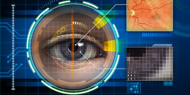
Examples of Computer Vision
You can probably name numerous examples of computer vision already, but just to highlight a couple:
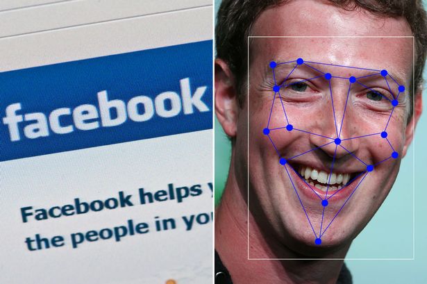
- Facebook and Google use sophisticated computer vision methods to perform facial recognition scans of photos that are uploaded to their servers. You've likely seen examples of this when Facebook automatically puts boxes around the faces of people in a picture, and asks if you'd like to tag certain individuals.
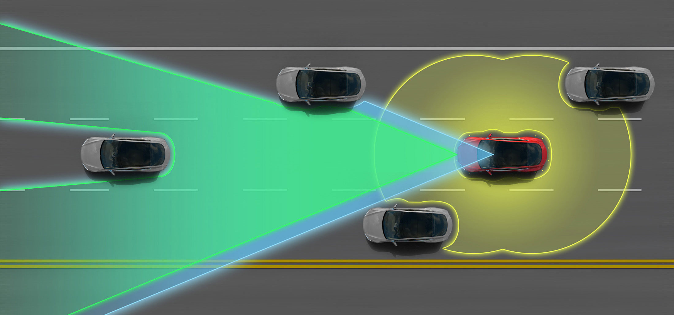
- Tesla Motors' "Autopilot" and other semi-autonomous vehicles use arrays of cameras to capture outside information, then process these photos using computer vision methods in order to pilot the vehicle. Google's experimental self-driving cars use similar techniques, but are fully autonomous.
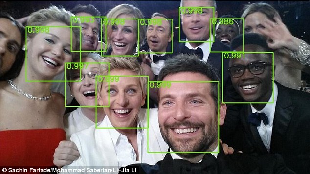
- The subarea of machine learning known as "deep learning" has exploded in the last five years, resulting in state-of-the-art image recognition capabilities. Google's DeepMind can recognize arbitrary images to an extraordinary degree, and similar deep learning methods have been used to automatically generate captions for these images.
This is all to underscore: computer vision is an extremely active area of research and application!
- Automated categorization and annotation of YouTube videos (identification of illegal content?)
- Analyzing photos on your smartphones
- License plate and facial recognition for law enforcement officials
- Disabled access to web technologies
- Virtual reality
Images and their Representations
From the perspective of the computer, the simplest constituent of an image is a pixel.
- pix: picture
- el: element
A pixel is a picture element.
- In a grayscale image, the pixel contains the intensity. Depending on the image format this may range from 0-1, 0-255, or be any floating point number.
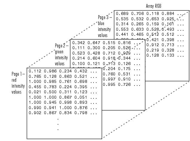
- In a color image, a pixel is (usually) a triple (red, green, blue) of color values where each color intensity ranges from 0-255 (24-bit color).
(There are many other image formats and representations, but they tend to be variations on this theme)
In either grayscale or color, the pixels are arranged in rectangular arrays, one for each color channel (1 for grayscale, 3 for RGB).
(What could these arrays possibly be in Python?)
Part 2: Loading and Manipulating Images
Let's jump in and get our hands dirty! First, let's use a relevant image:
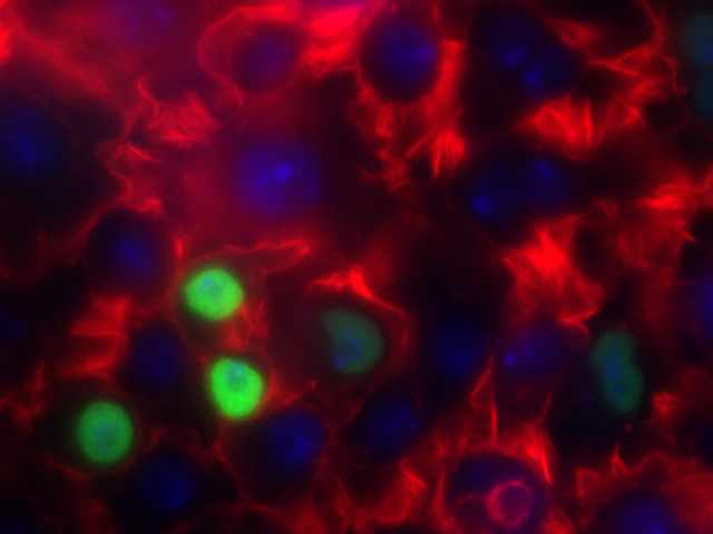
- Actin
- HSP27
- DAPI
I've stored this image in the course GitHub repository under lectures/ComputerVision ( https://github.com/eds-uga/cbio4835-fa18 ) if you're interested.
Here's how to load the images in Python:
%matplotlib inline
import numpy as np
import matplotlib.pyplot as plt
import matplotlib.image as mpimg
# Loads the image (just like a text file!)
img = mpimg.imread("ComputerVision/image1.png")

print(type(img))
Just a regular NumPy array!
Let's see if we can visualize it.
plt.imshow(img)

This shows the whole image, all three channels.
print(img.shape)
As evidenced by the .shape property of the NumPy array, there are three dimensions to this image:
- the first is height (or rows)
- the second is width (or columns)
- the third is color (or depth)
Each slice of the third dimension is a color channel, of which there are 3: one for red, one for green, and one for blue (hence: RGB).
We can plot them separately!
# First, separate out the channels.
r = img[:, :, 0]
g = img[:, :, 1]
b = img[:, :, 2]

# Now, plot each channel separately.
f = plt.figure(figsize = (12, 6))
f.add_subplot(1, 3, 1)
plt.imshow(np.array(r), cmap = "gray")
f.add_subplot(1, 3, 2)
plt.imshow(np.array(g), cmap = "gray")
f.add_subplot(1, 3, 3)
plt.imshow(np.array(b), cmap = "gray")

Image analysis of any kind is usually done on a single channel.
Since images are stored as NumPy arrays, all the usual NumPy functionality (besides slicing, as we saw earlier) is available to you.
- Want to compute the maximum and minimum pixel values in the images?
print(np.max(img))
print(np.min(img))
- Want to compute the average and median pixel values?
print(np.mean(img))
print(np.median(img))
- How about the median of each of the red, green, and blue channels separately?
print(np.median(r))
print(np.median(g))
print(np.median(b))
Converting Image Types
Recall that our img object was loaded from a PNG image; this is the only format type that Matplotlib natively supports (more on that later).
When you read an image into Python, it will automatically detect the format and read it into the closest approximate Python data format it can. However, you can always manually convert it once it's in Python.
For instance, we use a slightly different approach to instead read in our image as grayscale:
import scipy.ndimage as ndimg

img_gray = ndimg.imread("ComputerVision/image1.png", flatten = True)  # The "flatten" arg is critical
print(img_gray.shape)
Note how there are only 2 dimensions now--just a height and width.
There is no need for a 3rd dimension because there's only 1 channel: luminescence, or grayscale intensity.
plt.imshow(img_gray, cmap = "gray")

We can access individual pixels, just as you would individual elements of a matrix NumPy array (because that's all it is):
print(img_gray[100, 200])
print(img_gray[150, :])
print(np.max(img_gray[:, 400]))
If you so desire, you can even modify the pixel values directly, again just as you would for a regular NumPy array.
Fair warning: doing this alters the image! You may want to copy the image structure first...
for i in range(img_gray.shape[0]):
    for j in range(120, 130):
        img_gray[i, j] = 255

plt.imshow(img_gray, cmap = "gray")

Histograms
Another very useful way of obtaining information about an image is to view the histogram of pixel values.
You can do this regardless of whether it's a grayscale or RGB image, though in the latter case it's useful to plot the pixel values separated by channel.
First, let's re-import the image as grayscale and take a look at how the pixel values show up in a histogram:
img_gray = ndimg.imread("ComputerVision/image1.png", flatten = True)
_ = plt.hist(img_gray.flatten(), bins = 25)

This tells us some very useful information--primarily, that most of the pixel values are centered around what seems like a pretty low number (20-30), so by and large the image is very dark (which we saw).
There do seem to be a few light spots on an island around 120-140, but that's it.
Let's take a look now at each channel individually.
fig = plt.figure(figsize = (16, 4))
plt.subplot(131)
_ = plt.hist(r.flatten(), bins = 25, range = (0, 1), color = 'r')
plt.subplot(132)
_ = plt.hist(g.flatten(), bins = 25, range = (0, 1), color = 'g')
plt.subplot(133)
_ = plt.hist(b.flatten(), bins = 25, range = (0, 1), color = 'b')

Recall what each channel represented:
- Actin
- HSP27
- DAPI
There seems to be very little HSP27, while there is tons of actin and the quantity of DAPI falls somewhere in between.
...oh wait, did you see the scales for each one?
x = np.linspace(0, 1, 25)
plt.plot(x, np.histogram(r.flatten(), bins = 25)[0], color = 'r', label = 'Actin')
plt.plot(x, np.histogram(g.flatten(), bins = 25)[0], color = 'g', label = 'HSP27')
plt.plot(x, np.histogram(b.flatten(), bins = 25)[0], color = 'b', label = 'DAPI')
plt.legend()

So, yes:
- Clearly, very little HSP27 signal, relative to the other stains. Most of those pixels are black (0).
- There does seem to be a decent amount of DAPI signal, but like HSP27 it too drops off very quickly; not many DAPI pixels with brightness greater than 0.4 or so.
- The actin signal is probably the most interesting one, in that it's very diffuse--very few black (0) pixels, no white pixels either (1), but somewhere in between for the most part. This is fairly characteristic for actin.
Equalization
While we're on the topic of histograms, there is a convenient way to try and "reshape" the pixel histograms so as to make the resulting image a bit sharper. This is called histogram equalization.
The idea is simple enough: re-map the pixel values in the image so that the corresponding histogram is perfectly flat.
Basically it tries to fill in the "valleys" and flatten the "peaks" of the pixel histograms we saw earlier--this has the effect of bringing out very dim signal and dampening oversaturated signal.
Let's see an example, using one of the image channels.
from PIL import Image, ImageOps

img_pil = Image.open("ComputerVision/image1.png")
beq = ImageOps.equalize(img_pil.split()[2])

f = plt.figure(figsize = (12, 6))
f.add_subplot(1, 2, 1)
plt.imshow(b, cmap = 'gray')
f.add_subplot(1, 2, 2)
plt.imshow(np.array(beq), cmap = 'gray')

We can directly see why these two images look different (and, specifically, what histogram equalization did) by recomputing the channel histograms:
plt.plot(img_pil.split()[2].histogram(), 'b')
plt.plot(beq.histogram(), 'k')

Autocontrast
Autocontrast is another tool that modifies the pixel histograms to try and make the resulting images more viewable. In this case, the goal of autocontrast is to maximize (normalize) image contrast.
This function calculates a histogram of the input image, removes cutoff percent of the lightest and darkest pixels from the histogram, and remaps the image so that the darkest remaining pixel becomes black (0), and the lightest becomes white (255).
In essence, you choose some percentage cut-off (say: 50%, or 0.5), removes that fraction of pixels that are both darkest and lightest (assumes they're noise and throws them away), then remaps the remaining pixels.
Here's what it might look like:
bcon = ImageOps.autocontrast(img_pil.split()[2], 0.5)

f = plt.figure(figsize = (12, 6))
f.add_subplot(1, 2, 1)
plt.imshow(b, cmap = "gray")
f.add_subplot(1, 2, 2)
plt.imshow(np.array(bcon), cmap = "gray")

In this case, we're trying to chop off pixel values at both ends of the histogram (lightest and darkest) and reshuffling the others around to make them more visible, hopefully improving contrast.
The effects on the underlying histograms look like:
plt.plot(img_pil.split()[2].histogram(), 'r')
plt.plot(bcon.histogram(), 'k')

It closely mimics the original histogram, but because some values at the tails were thrown away, all the other values were reshuffled--you end up with more pixels some of the middle values, which is (presumably) the signal you're interested in.
Thresholding
Thresholding is the process by which you define a pixel threshold--say, the value 100--and set every pixel below that value to 0, and every pixel above that value to 255.
In doing so, you binarize the image, as each pixel takes on only one of two possible values.
Remember boolean indexing?
(head on over to Lecture 6 if you're a little fuzzy on the details)
In short, you can create masks based on certain boolean conditions so you can modify certain parts of the array while holding the others constant.
Here's the example straight from the lecture:
x = np.random.standard_normal(size = (7, 4))
print(x)
If we just want the positive numbers, we can define a mask using the condition you'd find in an if statement:
mask = x < 0  # For every element of x, ask: is it < 0?
print(mask)
The mask is just a bunch of True and False values.
Now we can use the mask to modify the parts of the original array that correspond to True in the mask:
x[mask] = 0.0
print(x)
Back to images! Let's use a threshold on our blue channel:
b_thresh = np.array(bcon) > 120  # Every pixel greater than 120 is "True", otherwise it's "False"

f = plt.figure(figsize = (12, 6))
f.add_subplot(1, 2, 1)
plt.imshow(np.array(bcon), cmap = "gray")
f.add_subplot(1, 2, 2)
plt.imshow(b_thresh, cmap = "gray")

Any ideas how we might, say, count the number of cells?
Part 3: Computer Vision in Python
There is an entire ecosystem of computer vision packages for Python.
Some are very general (a lot like scipy.ndimage and PIL) while some are very specific to certain classes of problems.
You could spend an entire career with just one or two of these packages, but very briefly I'll name a few of the most popular.
(We'll make use of some of them!)
scikit-image
![]()
If scipy.ndimage or PIL proves to be insufficient for your needs, this should be the first stop you take in looking for alternatives.
It has a wealth of general-purpose image processing routines built-in. It's actively developed and very easy to use, and integrates well with NumPy and SciPy.
It also comes with a bunch of basic tutorials and sample data to help you get your feet wet.
mahotas
This is another excellent general-purpose image processing library, though it has a slight preference for bio-imaging applications. After all, its author is a computational biologist!
Like scikit-image, it's actively developed, easy to use, and integrates fully with the NumPy + SciPy scientific computing environment for Python.
This is probably your first stop if you're looking for some basic bioimaging tools.
OpenCV

OpenCV (for "Open Computer Vision") is the Grand Daddy of image processing packages.
You'll want to use this if computer vision is a significant part of your day-to-day career. It's not for the faint of heart, however: it's a C++ library with Python bindings, which means you have to install from source, and that can be painful depending on how (un)comfortable you are with compiling things from scratch.
(though if you use the Anaconda distribution of Python, and you connect it to the conda-forge channel, you can download pre-built OpenCV packages that WAY SIMPLIFY this process)
That said, OpenCV has everything:
- automated image segmentation
- facial recognition
- video stabilization
- optical flow algorithms
- image stitching
- filtering
- warping
- matching
- deep learning
- ...
The list goes on and on.
It's well-maintained, well-documented, and while it can be a little tricky to use, it has a huge community of developers and users ready to help.
Like scikit-image, it also provides a ton of tutorials for typical use-cases, though OpenCV's definition of "typical" is a little different: they're actually pretty in-depth!
Administrivia
- Assignment 4 is due today!
- Project proposals are also due today!
Additional Resources
- Matplotlib image tutorial http://matplotlib.org/users/image_tutorial.html
- scikit-image http://scikit-image.org/
- mahotas http://mahotas.readthedocs.io/en/latest/
- OpenCV http://opencv.org/
- OpenCV Python tutorials http://docs.opencv.org/3.2.0/d6/d00/tutorial_py_root.html