Lecture 5: Modules, NumPy, and File I/O
CBIO (CSCI) 4835/6835: Introduction to Computational Biology
Overview and Objectives
So far, all the "data" we've worked with have been manually-created lists or other collections. A big part of your careers as computational scientists will involve interacting with data saved in files. Here we'll finally get to go over reading to and writing from the filesystem, and using much more advanced array structures to store the data. By the end of this lecture, you should be able to:
- Implement a basic file reader / writer using built-in Python tools
- Import and use Python modules
- Compare and contrast NumPy arrays to built-in Python lists
- Define "broadcasting" in the context of vectorized programming
- Use NumPy arrays in place of explicit loops for basic arithmetic operations
- Understand the benefits of NumPy's "fancy indexing" capabilities and its advantages over built-in indexing
Part 1: Interacting with text files
Text files are probably the most common and pervasive format of data. They can contain almost anything: weather data, stock market activity, literary works, raw web data.
On the biological end, they can contain things like sequence alignments, protein sequences, molecular structure information, and myriad other data.
Text files are also convenient for your own work: once some kind of analysis has finished, it's nice to dump the results into a file you can inspect later.
Reading an entire file
So let's jump into it! Let's start with something simple: a FASTA text file for the BRCA1 gene.
f = open("Lecture6/brca1.fasta", "r")
line = f.readline()
print(line)
f.close()
Aside
A quick review on FASTA files (we'll get into this more in a future lecture)
FASTA refers to software from 1985 for DNA and protein sequence alignment. The software is long obsolete, but its namesake lives on in the file format it used: FASTA-format.
A sequence in a FASTA file is represented as a series of lines.
- The first line starts with a greater-than carrot
>and contains a "human-readable" description of the sequence in the file. It usually contains an accession number for the sequence, and may contain other information as well.
- Following this line are sequences, using single-letter codes. Anything other than a valid sequence is traditionally ignored.
Code walkthrough
Back to the code, then. First, we have a function open() that accepts two arguments:
f = open("Lecture6/brca1.fasta", "r")
- The first argument is the file path. It's like a URL, except to a file on your computer. It should be noted that, unless you specify a leading forward slash
"/"(an absolute path), Python will interpret this path to be relative to wherever the Python script is that you're running with this command.
- The second argument is the mode. This tells Python whether you're reading from a file, writing to a file, or appending to a file. We'll come to each of these.
These two arguments are part of the function open(), which then returns a file descriptor. It's your key to accessing or modifying the contents of the file.
The next line is where the magic happens:
line = f.readline()
In this line, we're calling the method readline() on the file reference we got in the previous step. This method goes into the file, pulls out the first line, and sticks it in the variable line as one long string.
print(line)
...which we then simply print out.
Finally, the last and possibly most important line:
f.close()
This statement explicitly closes the file reference, effectively shutting the valve to the file.
Do not underestimate the value of this statement. There are weird errors that can crop up when you forget to close file descriptors. It can be difficult to remember to do this, though; in other languages where you have to manually allocate and release any memory you use, it's a bit easier to remember. Since Python handles all that stuff for us, it's not a force of habit to explicitly shut off things we've turned on.
Fortunately, there's an alternative those of us with bad short-term memory can use.
with open("Lecture6/brca1.fasta", "r") as f:
    line = f.readline()
    print(line)
This code works identically to the code before it. The difference is, by using a with block, Python intrinsically closes the file descriptor at the end of the block. Therefore, no need to remember to do it yourself! Hooray!
File modes
What was the "r" file mode from the open() call?
The "mode" is the way you tell Python exactly what you want to do with the file you're accessing. There are three modes:
"r"for read mode. The file will only be read from (it must already exist).
"w"for write mode. The file is created or truncated (anything already there is deleted) and can only be written to.
"a"for append mode. The file is created or appended to (does not delete or truncate any existing file) and can only be written to.
Manipulating Files
There are lots of other methods besides open(), close(), and readline() for tinkering with files.
read- return the entire file as a string (can also specify optional size argument)readlines- return lists of all lineswrite- writes a passed string to the fileseek- set current position of the file; seek(0) starts back at beginning
Which methods can be used in read mode? write mode? append mode?
What is the value of line?
f = open('Lecture6/brca1.fasta')
f.read()
line = f.readline()
print(line)
Hello....... Newline.
In Python, we've emphasized how whitespace is important. Recall that whitespace is defined as a character you can't necessary "see": tabs and spaces, for example.
There's a third character in the whitespace category: the newline character. It's what "appears" when you press the Enter key.
Internally, it's seen by Python as a character that looks like this: \n
But whenever you view plain text, the character is invisible. The only way you can tell it's there is by virtue of the fact that text is separated into lines.
However, when you're reading data in from files (and writing it out, too), you can't afford to ignore these newline characters. They can get you in a lot of trouble.
with open("Lecture6/brca1.fasta", "r") as f:
    for i in range(5):
        line = f.readline()
        print(line)
What's with the blank lines between each DNA sequence?
You can't see it, but there are newline characters at the ends of each of the lines. Those newlines, coupled with the fact that print() implicitly adds its own newline character to the end of whatever you print, means the Enter key was effectively pressed twice.
Hence, the blank line between each sequence.
So how can we handle this?
strip()
Strings in Python have a wonderful strip() function. It cuts off any whitespace on either end.
lots_of_whitespace = "\n\n          this is a valid string              \n"
print(lots_of_whitespace)
stripped = lots_of_whitespace.strip()
print(stripped)
strip() chops and chops from both ends of a string until it reaches non-whitespace characters.
Writing to files
We've seen reading from files. How about writing to them? (spoiler alert: newlines can be a pain here, too)
data_to_save = "This is important data. Definitely worth saving."
with open("outfile.txt", "w") as file_object:
    file_object.write(data_to_save)
You'll notice two important changes from before:
- Switch the
"r"argument in theopen()function to"w"(changing from reading to writing). - Call
write()on your file descriptor, and pass in the data you want to write to the file (in this case,data_to_save).
If you try this using a new notebook on JupyterHub (or on your local machine), you should see a new text file named "outfile.txt" appear in the same directory as your script. Give it a shot!
!cat outfile.txt
And there you have it. Some notes about writing files:
- If the file you're writing to does NOT currently exist, Python will try to create it for you. In most cases this should be fine
- If the file you're writing to DOES already exist, Python will overwrite everything in the file with the new content. As in, everything that was in the file before will be erased.
That second point seems a bit harsh, doesn't it? Luckily, there is recourse.
Appending to an existing file
If you find yourself in the situation of writing to a file multiple times, and wanting to keep what you wrote to the file previously, then you're in the market for appending to a file.
This works exactly the same as writing to a file, with one small wrinkle:
data_to_save = "This is ALSO important data. BOTH DATA ARE IMPORTANT."
with open("outfile.txt", "a") as file_object:
    file_object.write(data_to_save)
The only change that was made was switching the "w" in the open() method to "a" for append mode. If you look in outfile.txt, you should see both lines of text we've written.
!cat outfile.txt
Whoa, why are those two sentences scrunched right up against each other?
Newlines strike again! When you're writing to a file, you'll need to explicitly put in the newlines when you want something to go on a separate line.
data_to_save = "This is the first line.\n"
with open("outfile.txt", "w") as file_object:  # "w" mode
    file_object.write(data_to_save)

more_data = "Here's the second line.\n"
with open("outfile.txt", "a") as file_object:  # "a" mode
    file_object.write(more_data)
What is in outfile.txt?
!cat outfile.txt
Some notes about appending to a file.
- If the file does NOT already exist, then using "a" in
open()is functionally identical to using "w".
- You only need to use append mode if you closed the file descriptor to that file previously. If you have an open file descriptor, you can call
write()multiple times; each call will append the text to the previous text. It's only when you close a descriptor, but then want to open up another one to the same file, that you'd need to switch to append mode.
Part 2: Importing Modules
Python comes with a number of packages that provide additional functionality. These are called modules.
Any Python file is a module. The code in these modules can be included in your Python program using the import command.
import this
Lots of other packages that come default with Python:
import random   # For generating random numbers
import os       # For interacting with the filesystem of your computer
import sys      # Helps with customizing the behavior of your Python program
import re       # For regular expressions. Unrelated: https://xkcd.com/1171/
import datetime # Helps immensely with determining the date and formatting it
import math     # Gives some basic math functions: trig, factorial, exponential, logarithms, etc.
If you are so inclined, you can see the full Python default module index here: https://docs.python.org/3/py-modindex.html.
Keep in mind--those are just the packages that come with Python. These constitute a teeny tiny drop in the proverbial bucket when you include 3rd party packages available through the Python Package Index. At posting, PyPI was tracking 96,893 Python packages.
Once you've imported a package, all the variables and functions in the module are accessible through the module object.
import math
print(math.pi)
print(pi)
Namespaces
A namespace in Python, without going into too much detail (yet), is the collection of variables / objects / named things that you have at your disposal.
When you get a NameError like in the previous slide when trying to reference pi, this is because pi is not defined in that particular namespace; instead, it's defined in the math namespace.
Of course, you could always define your own variable pi:
pi = 3.14  # an approximation

print(math.pi)
print(pi)
These are two different variables, because they exist in different namespaces. They just happen to have the same names.
If, on the other hand, you wanted to import the math.pi variable directly into the full namespace, you could adjust the import statement to look like this:
from math import pi
print(pi)
By importing pi directly into the full namespace, it has the same effect as reassigning our previous variable pi--as in, it got wiped out by this new one.
This is why namespaces are useful--they can differentiate between functions and variables with the same name.
Part 3: NumPy
NumPy, or Numerical Python, is an incredible library of basic functions and data structures that provide a robust foundation for computational scientists.
Put another way: if you're using Python and doing any kind of math, you'll probably use NumPy.
At this point, NumPy is so deeply embedded in so many other 3rd-party modules related to scientific computing that even if you're not making explicit use of it, at least one of the other modules you're using probably is.
NumPy's core: the ndarray
NumPy, or Numerical Python, is an incredible library of basic functions and data structures that provide a robust foundation for computational scientists.
As an example: remember when we spoke about lists-of-lists? That's pretty much the only way we can create matrices using built-in Python data structures.
matrix = [[ 1, 2, 3],
          [ 4, 5, 6],
          [ 7, 8, 9] ]
print(matrix)
Indexing would still work as you would expect, but looping through a matrix--say, to do matrix multiplication--would be laborious and highly inefficient.
By contrast, in NumPy, we have the ndarray structure (short for "n-dimensional array") that is a highly optimized version of Python lists, perfect for fast and efficient computations. To make use of NumPy arrays, import NumPy (it's installed by default in Anaconda, and on JupyterHub):
import numpy
Now just call the array method using our list from before!
arr = numpy.array(matrix)
print(arr)
The variable arr is a NumPy array version of the previous list-of-lists!
To reference an element in the array, just use the same notation we did for lists:
arr[0] # row 0
arr[2][2] # row 2, column 2
You can also separate dimensions by commas, if you prefer:
arr[2, 2]
Part 4: Vectorized Arithmetic
"Vectorized arithmetic" refers to how NumPy allows you to efficiently perform arithmetic operations on entire NumPy arrays at once, as you would with "regular" Python variables (like ints and floats).
For example: let's say I want to square every element in a list of numbers.
# Define our list:
our_list = [5, 10, 15, 20, 25]
# Write a loop to square each element:
for i in range(len(our_list)):
    # Reassign each element to be its own square.
    our_list[i] = our_list[i] ** 2
print(our_list)
Sure, it works. But you might have a nagging feeling in the back of your head that there has to be an easier way...
With lists, unfortunately, there isn't one. However, with NumPy arrays, there is! And it's exactly as intuitive as you'd imagine!
# Define our list:
our_list = [5, 10, 15, 20, 25]
# Convert it to a NumPy array (this is IMPORTANT)
our_list = numpy.array(our_list)
our_list = our_list ** 2
# Yep, we just squared the WHOLE ARRAY. And it works how you'd expect!
print(our_list)
NumPy knows how to perform element-wise computations across an entire NumPy array. Whether you want to add a certain quantity to every element, subtract corresponding elements of two NumPy arrays, or square every element as we just did, it allows you to do these operations on all elements at once, without writing an explicit loop!
Operations involving arrays on both sides of the sign will also work (though the two arrays need to be the same length).
For example, adding two vectors together:
import numpy as np  # A common convention with NumPy.

x = np.array([1, 2, 3])
y = np.array([4, 5, 6])
z = x + y
print(z)
Works exactly as you'd expect, but no [explicit] loop needed.
The key to making vectorized programming work? Broadcasting.
zeros = np.zeros(shape = (3, 4))
print(zeros)
zeros += 1   # Just add 1.
print(zeros)
In this example, the scalar value 1 is broadcast to all the elements of zeros, converting the operation to element-wise addition.
This all happens under the NumPy hood--we don't see it! It "just works".
...most of the time, anyway. If you see an error that looks like this:
x = np.zeros(shape = (3, 3))
y = np.ones(4)
x + y
It's because Python couldn't figure out how to properly broadcast the NumPy arrays you were using.
(But on some intuitive level, this hopefully makes sense: there's no reasonable arithmetic operation that can be performed when you have one $3 \times 3$ matrix and a vector of length 4. So if you get this error, check your dimensions!)
Part 5: Indexing and Slicing
Remember indexing and slicing with Python lists?
li = ["this", "is", "a", "list"]
print(li)
print(li[1:3])  # Print element 1 (inclusive) to 3 (exclusive)
print(li[2:])   # Print element 2 and everything after that
print(li[:-1])  # Print everything BEFORE element -1 (the last one)
With NumPy arrays, all the same functionality you know and love from lists is still there.
x = np.array([1, 2, 3, 4, 5])
print(x)
print(x[1:3])
print(x[2:])
print(x[:-1])
These operations all work whether you're using Python lists or NumPy arrays.
The first place in which Python lists and NumPy arrays differ is when we get to multidimensional arrays (including matrices, but possibly with three, four, or more dimensions).
When you index NumPy arrays, the nomenclature used is that of an axis: you are indexing specific axes of a NumPy array object (rows, columns, etc are axes).
To illustrate with an example:
python_matrix = [ [1, 2, 3], [4, 5, 6], [7, 8, 9] ]
print(python_matrix)
numpy_matrix = np.array(python_matrix)
print(numpy_matrix)
You can query the number of axes in a NumPy array with the .shape attribute:
print(numpy_matrix.shape)
The .shape attribute tells you two things:
1: How many axes there are. This number is len(ndarray.shape), or the number of elements in the tuple returned by .shape. In our above example, numpy_matrix.shape would return (3, 3), so it would have 2 axes (since there are two numbers--both 3s).
2: How many elements are in each axis. In our above example, where numpy_matrix.shape returns (3, 3), there are 2 axes (since the length of that tuple is 2), and both axes have 3 elements (hence the numbers--3 elements in the first axis, 3 in the second).
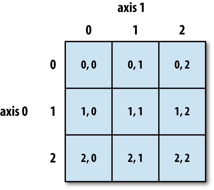
Here's the breakdown of axis notation and indices used in a 2D NumPy array:
As with lists, if you want an entire axis, just use the colon operator all by itself:
x = np.array([ [1, 2, 3], [4, 5, 6], [7, 8, 9] ])
print(x)
print(x[:, 1]) # Take ALL of axis 0, and one index of axis 1.
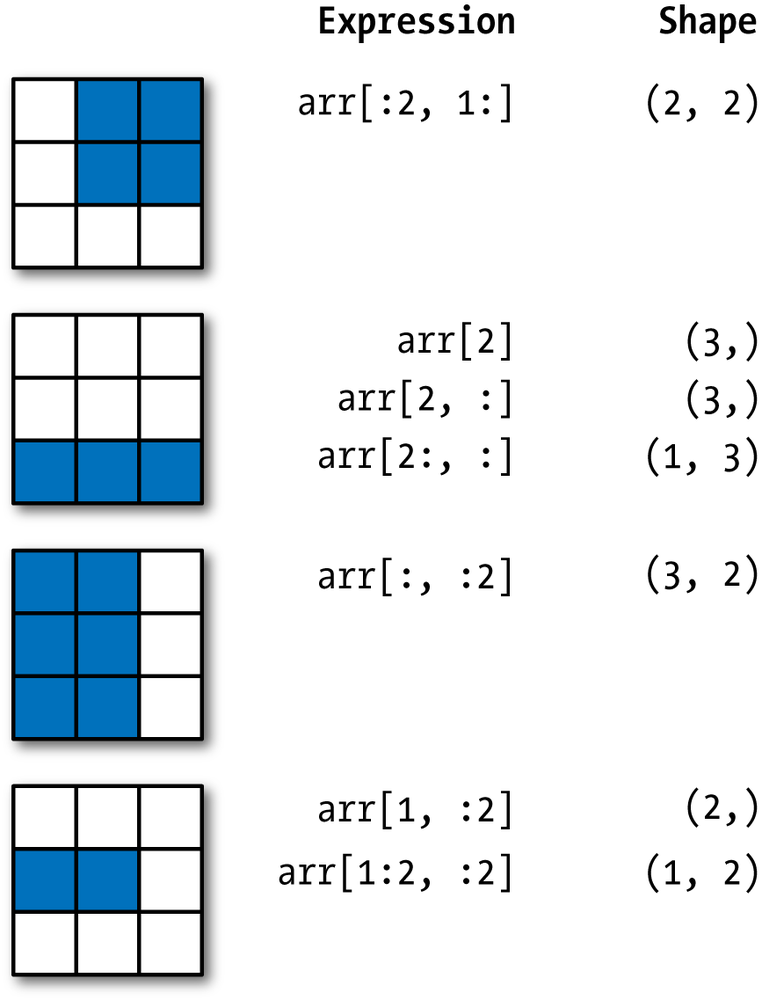
Here's a great visual summary of slicing NumPy arrays, assuming you're starting from an array with shape (3, 3):
STUDY THIS CAREFULLY. This more or less sums up everything you need to know about slicing with NumPy arrays.
Depending on your field, it's entirely possible that you'll go beyond 2D matrices. If so, it's important to be able to recognize what these structures "look" like.
For example, a video can be thought of as a 3D cube. Put another way, it's a NumPy array with 3 axes: the first axis is height, the second axis is width, and the third axis is number of frames.
video = np.empty(shape = (1920, 1080, 5000))

print("Axis 0 length:", video.shape[0])  # How many rows?
print("Axis 1 length:", video.shape[1]) # How many columns?
print("Axis 2 length:", video.shape[2])  # How many frames?
del video # deletes a variable; convenient for LARGE variables
The number of axes can go as high as you want! The indexing remains the same!
If in doubt: once you index the first axis, the NumPy array you get back has the shape of all the remaining axes.
example = np.empty(shape = (3, 5, 9))
print(example.shape)
sliced = example[0]  # Indexed the first axis.
print(sliced.shape)
sliced_again = example[0, 0]  # Indexed the first and second axes.
print(sliced_again.shape)
Notice how the number "9", initially the third axis, steadily marches to the front as the axes before it are accessed.
Part 6: Fancy Indexing
Hopefully you have at least an intuitive understanding of how indexing works so far. If not, ask!
"Fancy indexing" applies to a couple situations, like the following:
- I have a 2D NumPy array (2 axes) where each row contains the $x$, $y$, and $z$ coordinates of atoms in a protein. I want to access just the elements of the array with $x$ values that are negative (less than 0).
- I can access elements one at a time using their integer index, but someone gave a whole list of integer indices (indexes?) into a genome. That list is also re-ordered to reflect priority; how can I pull out all those elements by their index at once, and in the prescribed order?
These are all operations you could do with a loop!...or several. But they are so much faster and more efficient with fancy indexing.
First, let's say you want data out of your NumPy array that satisfy a certain condition. Therefore, you don't care about the numerical index, you just want very specific data (say, everything less than 0).
# Let's create some "toy" data.

x = np.random.standard_normal(size = (7, 4))
print(x)
This is randomly generated data, yes, but it could easily be 7 data points in 4 dimensions. That is, we have 7 observations of variables with 4 descriptors. Perhaps it's
- 7 people who are described by their height, weight, age, and 40-yard dash time, or
- Data on 7 video games, each described by their PC Gamer rating, Steam downloads count, average number of active players, and total cheating complaints, or
- A single atom's $x$, $y$, and $z$ coordinates at 7 different time points $t$
- ...insert your own example here!
If the example we're looking at is the video game scenario from the previous slide, then we know that any negative numbers are junk. After all, how can you have a negative rating? Or a negative number of active players?
Perhaps some goofy players decided to make bogus ratings. Funny to them, perhaps, but not exactly useful to you when you're trying to write an algorithm to recommend games to players based on their ratings. So, you have to "clean" the data a bit.
So our first course of action might be to set all negative numbers in the data to 0.
We could potentially set up a pair of loops--you should know how to do this!--but it's much easier (and faster) to use boolean indexing.
First, we create a mask. This is what it sounds like: it "masks" certain portions of the data we don't want to change (in this case, all the numbers greater than 0, since we're assuming they're already valid).
mask = x < 0
print(mask)
Just for your reference, here's the original data: notice how, in looking at the data below and the boolean mask above, all the spots where there are negative numbers also correspond to "True" in the mask?
print(x)
Now, we can use our mask to access only the indices we want to set to 0.
x[mask] = 0  # See that indexing notation?
print(x)
voilà! Every negative number has been set to 0, and all the other values were left unchanged. Now we can continue with whatever analysis we may have had in mind.
Important conceptual note: We just indexed a NumPy array with another NumPy array. It was full of booleans, but this concept of "indexing an array with another array" will be important in this last "fancy indexing" approach...
In addition to indexing NumPy arrays with boolean arrays (masks), you can also index them with NumPy arrays of integers--as in, the things we were originally taught to use when indexing collections!
Before you go down the Indexing Inception rabbit hole, just keep in mind: it's basically like slicing, but you're condensing the ability to perform multiple slicings all at one time, instead of one at a time.
Where we might have said x[0:3] (out loud: "pull out elements of x at positions 0 up to 3"), we could instead use a NumPy array of the form indexes = np.array([0, 1, 2]), and then do x[indexes]. It would achieve the same effect, but it gives us a TON more flexibility since we can change the form of that indexing array.
Now, to demonstrate: let's build a 2D array that, for the sake of simplicity, has across each row the index of that row.
matrix = np.empty(shape = (8, 4))
for i in range(8):
    matrix[i] = i  # Broadcasting is happening here!
print(matrix)
We have 8 rows and 4 columns, where each row is a 4-element vector of the same value repeated across the columns, and that value is the index of the row.
In addition to slicing and boolean indexing, we can also use other NumPy arrays to very selectively pick and choose what elements we want, and even the order in which we want them.
Let's say I want rows 7, 0, 5, and 2. In that order.
# Here's my "indexing" array--note the order of the numbers.
indices = np.array([7, 0, 5, 2])

# Now, use it as an index to "matrix" from earlier.
print(matrix[indices])
Ta-daaaa!
Row 7 shows up first (we know that because of the straight 7s), followed by row 0, then row 5, then row 2. You could get the same thing if you did matrix[7], then matrix[0], then matrix[5], and finally matrix[2], and then stacked the results into that final matrix. But this just condenses all those steps.
Fancy indexing can be tricky at first, but it can be very useful when you want to pull very specific elements out of a NumPy array and in a very specific order.
Fancy indexing is super advanced stuff, but if you put in the time to practice, it can all but completely eliminate the need to use loops.
Don't worry if you're confused right now. That's absolutely alright--this lecture and last Friday's are easily the most difficult if you've never done any programming before. Be patient with yourself, practice what you see in this lecture using the code (and tweaking it to see what happens), and ask questions!
Review Questions
1: Given some arbitrary NumPy array and only access to its .shape attribute (as well as its elements), describe (in words or in Python pseudocode) how you would compute exactly how many individual elements exist in the array (as in, you can't use .size).
2: Broadcasting hints that there is more happening under the hood than meets the eye with NumPy. With this in mind, do you think it would be more or less efficient to write a loop yourself in Python to add a scalar to each element in a Python list, rather than use NumPy broadcasting? Why or why not?
3: I have a 2D matrix, where the rows represent individual gamers, and the columns represent games. There's a "1" in the column if the gamer won that game, and a "0" if they lost. Describe how you might use boolean indexing to select only the rows corresponding to gamers whose average score was above a certain threshold.
4: Show how you could reverse the elements of a 1D NumPy array using one line of code, no loops, and fancy indexing.
5: Let's say I create the following NumPy array: a = np.zeros(shape = (100, 50, 25, 10)). What is the shape of the resulting array when I index it as follows: a[:, 0]?
6: NumPy arrays have an attribute called .shape that will return the dimensions of the array in the form of a tuple. If the array is just a vector, the tuple will only have 1 element: the length of the array. If the array is a matrix, the tuple will have 2 elements: the number of rows and the number of columns. What will the shape tuple be for the following array: tensor = np.array([ [ [1, 2], [3, 4] ], [ [5, 6], [7, 8] ], [ [9, 10], [11, 12] ] ])
7: Vectorized computations may seem almost like magic, and indeed they are, but at the end of the day there has to be a loop somewhere that performs the operations. Given what we've discussed about interpreted languages, compiled languages, and in particular how the delineations between the two are blurring, what would your best educated guess be (ideally without Google's help) as to where these loops actually happen that implemented the vectorized computations?
8: Does the answer to the above question change your perspective on whether Python is a compiled or an interpreted language?
9: Using your knowledge of slicing from a few lectures ago, and your knowledge from this lecture that NumPy arrays also support slicing, let's take an example of selecting a sub-range of rows from a two-dimensional matrix. Write the notation you would use for slicing out / selecting all the rows except for the first one, while retaining all the columns (hint: by just using : as your slicing operator, with no numbers, this means "everything").
Administrivia
- Biology Thursday!
- Assignment 1 is due Thursday! Any questions?
- Assignment 2 will also be out Thursday!
- Previous experience teaching this material suggests indexing is easily the most difficult, but also the most important, programming aspect of Python. So if you're having trouble with the material, please ask!
Additional Resources
- Matthes, Eric. Python Crash Course, Chapter 10. 2016. ISBN-13: 978-1593276034
- Model, Mitchell. Bioinformatics Programming Using Python, Chapter 2. 2010. ISBN-13: 978-0596154509
- NumPy Quickstart Tutorial: https://docs.scipy.org/doc/numpy-dev/user/quickstart.html
- NumPy documentation on array broadcasting http://docs.scipy.org/doc/numpy/user/basics.broadcasting.html
- NumPy documentation on indexing http://docs.scipy.org/doc/numpy/user/basics.indexing.html
- Broadcasting Arrays in NumPy. http://eli.thegreenplace.net/2015/broadcasting-arrays-in-numpy/