Lecture 16: Computational Structural Biology

CBIO (CSCI) 4835/6835: Introduction to Computational Biology

Overview and Objectives

Even though we're "officially" moving off modeling, we're still using similar techniques to study protein structure dynamics--how they fold, how they interact, how they bind, how they function. Proteins are enormously complex and modeling them requires answering a range of questions. By the end of this lecture, you should be able to

• Discuss the trade-offs of different strategies to represent protein structure and function
• Convert from Cartesian to generalized coordinates
• Explain dihedral angles and their role in verifying a valid generalized coordinate transformation
• Define a protein trajectory and its role in simulating protein function
• Create a trajectory covariance matrix and find its primary modes of variation
• Explain principal components analysis and singular value decomposition, and how to use these techniques to analyze protein trajectory data

Part 1: What is computational structural biology?

Not so dissimilar from computational modeling--basically a different side of the same coin.

Definition 1: Development and application of theoretical, computational, and mathematical models and methods to understand the biomolecular basis and mechanisms of biomolecular functions.

Definition 2: Understanding the fundamental physical principles that control the structure, dynamics, thermodynamics, and kinetics of biomolecular systems.

Basically, modeling of molecular structure.

Historical Perspective

• 1946: Molecular mechanics calculations

• 1950: $\alpha$-helices and $\beta$-strads proposed by Pauling

• 1960: force fields)

• 1969: Levinthal's paradox of protein folding

• 1970: first molecular dynamics simulation of biomolecules

• 1971: The Protein Data Bank

• 1998: Ion channel crystal structure

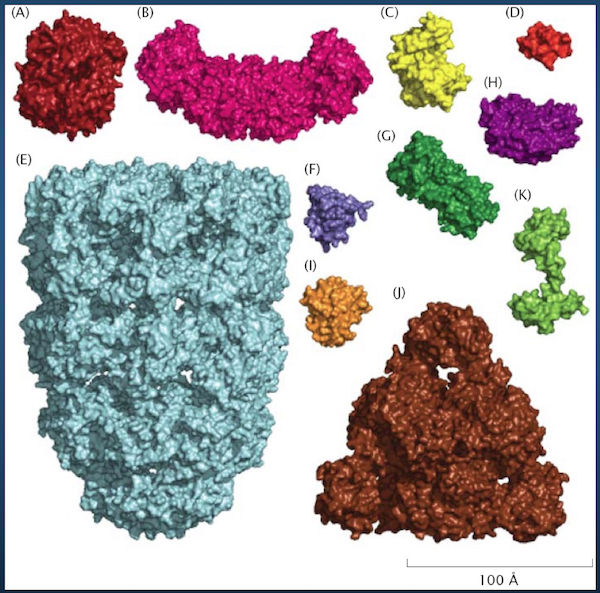
Available Resources

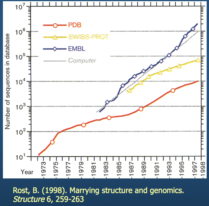
As I'm sure everyone is aware: both computing technology and available storage have grown exponentially over the last few decades. This has enabled us to stockpile structure data and analyze it.

PBD: Protein Data Bank

If you haven't, I encourage you to check out this website.

• Contains 3D structure data for hundreds of thousands of molecules

• Builds multiple structure viewers into the browser (don't need to install separate programs to view the molecules)

• Has built-in tools for sequence and structure alignment, among others

We'll come back to this (specifically, the eponymous PDB structure file).

Timescales

Of course, obtaining the structure of a molecule is a challenge (i.e. X-ray crystallography), but what we're discussing here is what we do after obtaining the structure information.

Note from the previous definitions a common thread: dynamics, kinetics, and thermodynamics. We're interested in how structure changes--i.e., a notion of time.

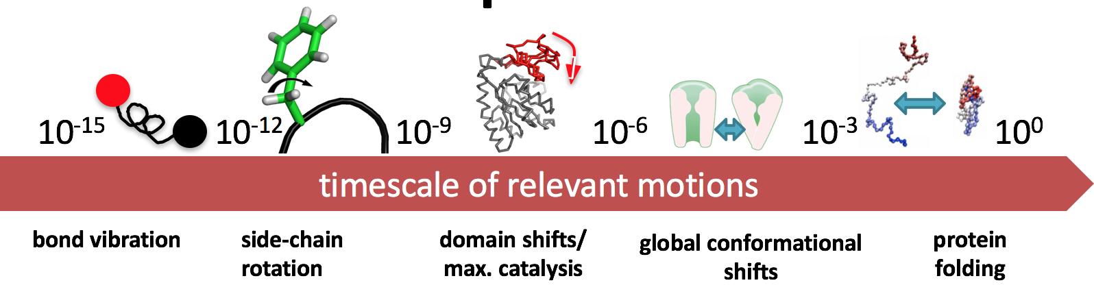
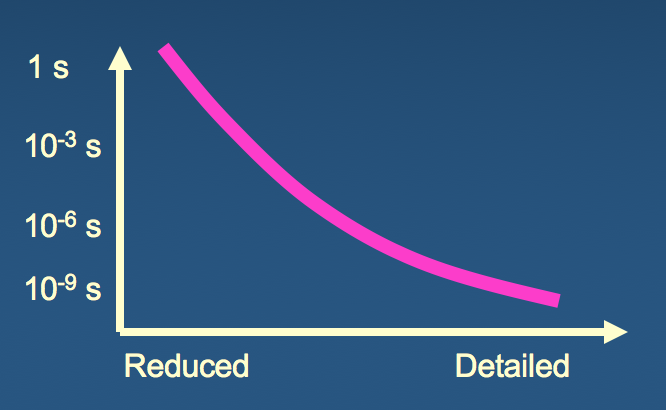
There's a trade-off in terms of resolution and speed.

• If you want to simulate bond vibration ($10^{-15}$), you'll need quite a few simulations to obtain a physically meaningful result

• If you want to simulate protein folding ($10^{0}$), you'll need a creative way to introduce some detail.

What are the minimal ingredients of a simplified, but physically meaningful, model of structure?

Part 2: Protein Structure Basics

First, we need to go over some preliminary background regarding protein structure before we get into how to model it.

As you all know, there is a hierarchy in protein structure.

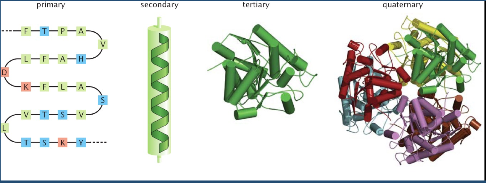
This hierarchy is where structural variability--and ultimately, function--comes from.

Of course, polypeptide chains have potentially enormous variability (recall Levinthal's paradox).

There are "only" 20 amino acids, but accounting for their possible combinations, in addition to bond lengths, bond angles, and side chains exponentially increases the number of variables to consider.

We need a way of representing proteins from a modeling standpoint.

Generalized Coordinates

One way to represent a protein is to use our old friend and mainstay, Cartesian coordinates.

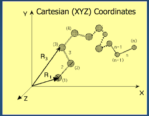
• Each atom in the backbone is represented as a 3D vector $R_i$
• The location of the $i^{th}$ atom with respect to the fixed frame XYZ is $R_i$
• What is the fixed frame XYZ?

Even better than Cartesian coordinates is generalized coordinates: we throw out absolute XYZ space for a representation of the polypeptide in an arbitrary location.

Instead of recording absolute spatial coordinates of atoms, we record bonds, bond angles, and dihedral angles.

Degrees of Freedom

The concept of degrees of freedom is an important one: this is basically the number of parameters that make up the system or model you're examining. Put another way, it's the number of "knobs" you can turn to get a unique configuration.

In generalized coordinates, how many degrees of freedom are there? Put another way, how many values do we need to specify, assuming $N$ backbone atoms, to fully characterize the 3D structure of a polypeptide?

• Bonds: $N - 1$ (do you see why?)

• Bond angles: $N - 2$ (do you see why?)

• Dihedral angles: $N - 3$ (do you see why?)

Total: $3N - 6$ (+ 6 external degrees of freedom: 3 translation, 3 rotation)

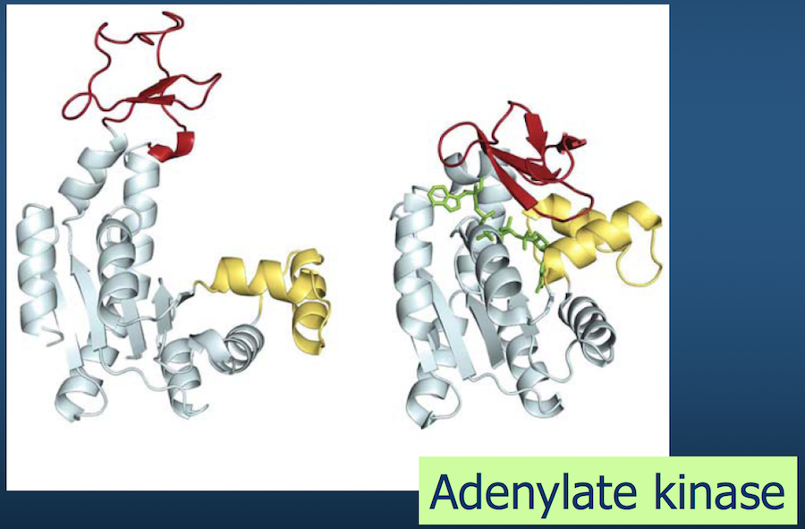
Molecule Movement

Of all the $3N - 6$ parameters in a generalized coordinate system, bond rotations (i.e. changes in dihedral angles) are the softest, and are primarily responsible for the protein's functional motions.

• Fluctuations around isomeric states near the native state

• Jumps between isomeric states

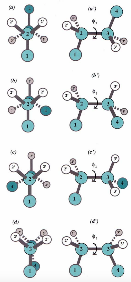
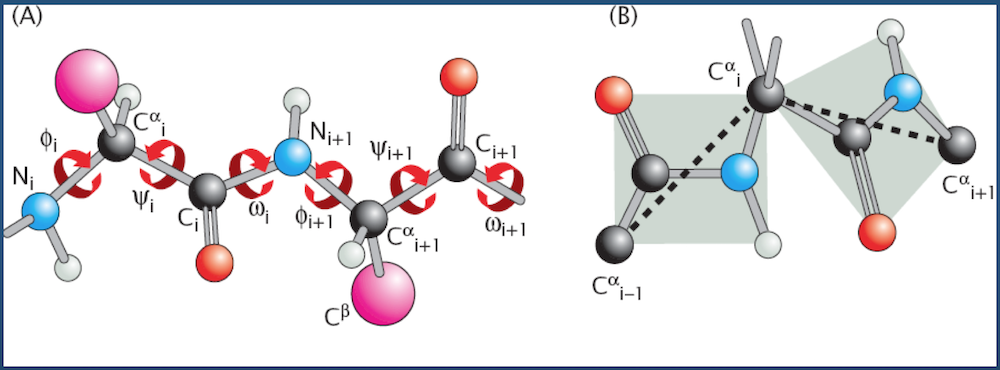
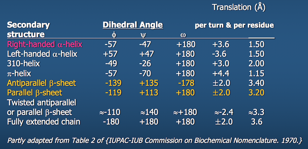
Dihedral angles

These torsional bonds have names: the $\phi$, $\psi$, and $\omega$ angles, though any angle with the $\phi$ prefix is understood to be a dihedral angle.

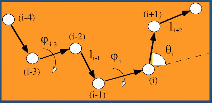
Cartesian to Generalized Coordinates

A quick primer on converting from absolute (Cartesian) coordinates to the more algorithmically-favorable generalized coordinates.

• Input: 3D Cartesian coordinates for $N$ atoms ${R_1 = (x_1, y_1, z_1), R_2 = (x_2, y_2, z_2), ..., R_N = (x_N, y_N, z_N)}$
• Output: Generalized coordinates for
  • $N - 1$ bonds $(l_2, l_3, ..., l_N)$
  • $N - 2$ bond angles $(\theta_2, \theta_3, ..., \theta_{N - 1})$
  • $N - 3$ dihedral angles $(\phi_3, \phi_4, ..., \phi_{N - 1})$

(the bond vector $l_i$ points from atom $i - 1$ to atom $i$; hence, we start with bond $l_2$)

Let's say you have a molecule with 4 atoms, $R_1$ through $R_4$ that each have their own $(x, y, z)$ coordinates.

• First, we calculate the bonds: $l_k = |R_k - R_{k - 1}|$

• Next, we calculate the bond angles: $\theta_k = \theta_k (R_{k - 1}, R_k, R_{k + 1}) = arccos\left( \frac{l_k \cdot l_{k + 1}}{|l_k \cdot l_{k + 1}|} \right)$

• Finally, the dihedral angles $\phi_k = \phi_k (R_{k - 2}, R_{k - 1}, R_k, R_{k + 1}) = sign [ arccos(-n_{k - 1} \cdot l_{k + 1})] arccos(-n_{k - 1} \cdot n_k)$

where $n_k$ is the unit vector that is perpendicular to the plane created by $l_k$ and $l_{k + 1}$. You can compute this vector by computing $n_k = \frac{l_k \times l_{k + 1}}{| l_k \times l_{k + 1} |}$

• $\times$ denotes an outer product, while $\cdot$ is an inner product
• $sign$ just means it takes the + or - from the resulting calculation

Conformational Space

Given these parameters, how many possible different conformations are there for a given $N$-atom protein?

Infinitely many.

Or, in discrete space, a whole freakin' lot.

Ramachandran Plots

Luckily...

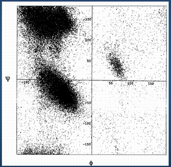
Ramachandran plot for 4 residue types:

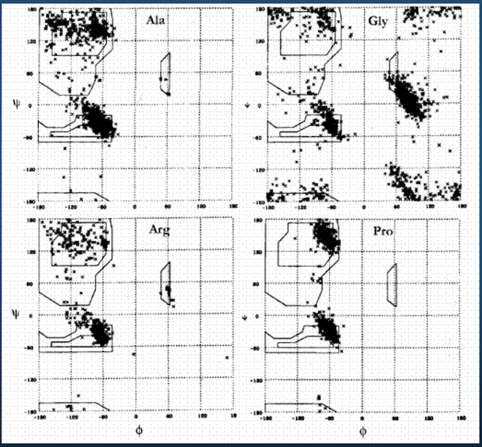
Upshot: even though there potentially infinitely-many conformations, real-life proteins seem to inhabit a very small space of conformational possibilities.

Part 3: Trajectories

At this point, we understand how to describe a polypeptide in space. Now we want to see what it does over time in some kind of environment.

This addition of time generates what is called a trajectory of the polypeptide, giving us insight into its function.

For a single residue $R_1$ (not to be confused with our definition of $R_1$ as the 3D Cartesian coordinates of an atom previously in this lecture), its trajectory looks something like this:

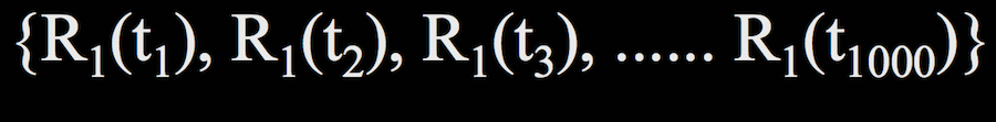
where $t_1$ through $t_{1000}$ are all the time points at which we evaluate the structure.

We're basically solving $F = ma$ for every atom in a residue at each time point; done over enough time points, we can start to see larger, coordinated behavior emerge.

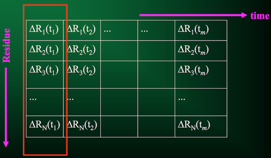
Of course, that's just for 1 residue. A protein usually has quite a few residues, in which case the trajectory would look something like this:

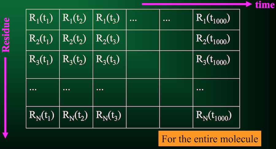
From this information, we can compute a few critical quantities.

The average position vector for $R_1$ is written as $ < R_1 > $. This is simply the average over all time points $t$.

From this quantity, we can compute the instantaneous fluctuation vector $\Delta R_1(t_i)$ at a specific time point $t_i$: $R_1(t_i) - < R_1 > $

Cross-correlation between fluctuation vectors of residues $R_i$ and $R_j$: $<\Delta R_i \cdot \Delta R_j> = \frac{1}{m} \sum_{k = 1}^m \Delta R_i (t_k) \cdot \Delta R_j (t_k)$

When $i = j$, this reduces to mean-square fluctuation.

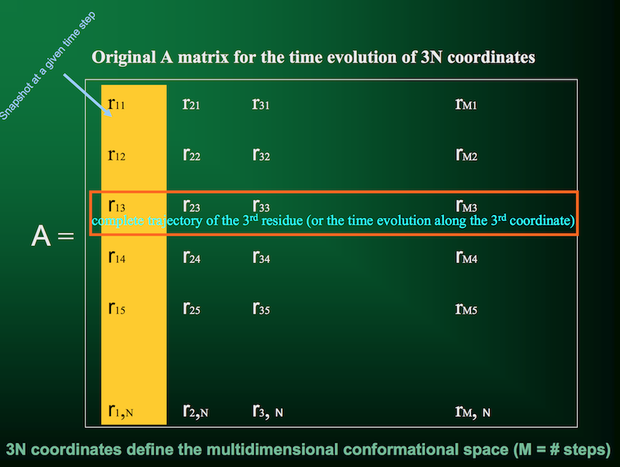
If we compute cross-correlations for all pairs of residues in the protein, this gives us the covariance matrix.

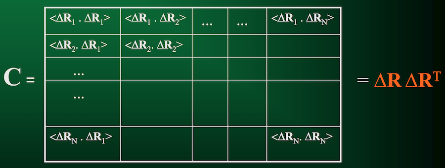
As the name implies, this matrix quantifies how each residue in a protein co-varies with each other residue over the duration of the trajectory.

Long-term Dynamics

The covariance matrix is a crucial component to understanding long-term dynamics of a protein.

After all, we're not necessarily interested in what happens between individual femtoseconds, but we need enough femtoseconds to be able to observe cooperative, global behavior in the protein.

But how do we uncover these dynamics from a covariance matrix?

Anyone remember Principal Components Analysis (PCA)?

Principal Components Analysis (PCA)

PCA is the most familiar of a family of analysis methods, collectively called dimensionality reduction techniques.

You can think of PCA (and really, any dimensionality reduction technique) as a sort of compression algorithm: condensing your existing data into a more compact representation, in theory improving interpretability of the data and discarding noise while maintaining the overall original structure.

Each algorithm goes about this process a little differently. PCA is all above maximizing variance.

Given some data, PCA tries to find new axes for the data. These axes are chosen to "maximize the variance in the data"--a complicated way of saying that it draws new coordinate axes to capture the directions in which the data move the most.

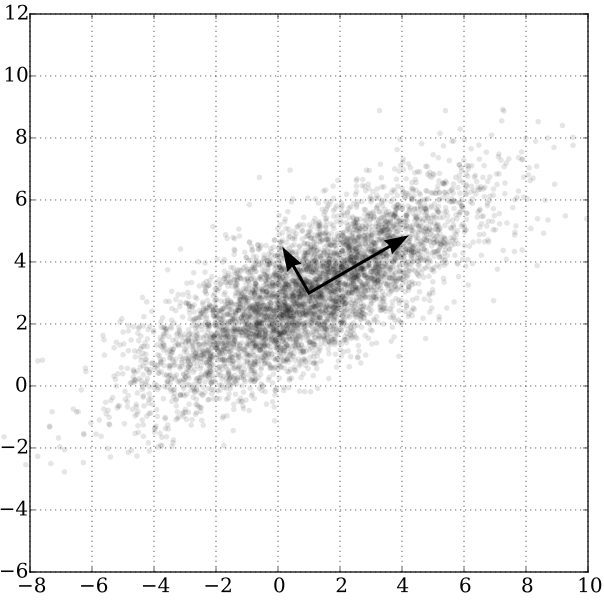
Once you have these "principal components", you can then choose to keep only the top handful--theoretically maintaining the majority of the variability in the data, but with considerably fewer data points.

This is precisely how we want to analyze our trajectory data. After all:

• Proteins, especially proteins we're really interested in, are likely quite large: several thousands of residues

• The number of trajectory snapshots required to observe long-term dynamics are probably on the order of millions, if not billions.

• A trajectory covariance matrix that's $N \times N$ is not going to be trivial to compute.

• But as we saw with Ramachandran plots, there are probably some patterns to how proteins behave. PCA can help discover those patterns.

Eigen-decomposition

We can rewrite the form of the covariance matrix $C$ as $C = U \Lambda U^{-1}$

• $U$ is the matrix of row-based eigenvectors
• $\Lambda$ is the diagonal matrix of eigenvalues
• $U^{-1} = U^T$

Cool. What do these mean?

Let's reorganize the equation a bit to gain some intuition about these quantities.

• When we first defined $C$ a few slides ago, we also said it could be written as $< \Delta R \Delta R^T >$.

• Using that notation, we'll substitute into the original eigen-decomposition equation: $< \Delta R \Delta R^T > = U \Lambda U^T$

• Since the $\Lambda$ matrix is diagonal (meaning the diagonal elements are the eigenvalues, and all the off-diagonal elements are 0), we can rewrite this matrix as an outer product of the same vector with itself: $q \times q^T$

• Now we have $< \Delta R \Delta R^T > = U q q^T U^T$, or $< \Delta R \Delta R^T > = (Uq)(Uq)^T$

We have an exact correspondence: $\Delta R = Uq$

• The $i^{th}$ eigenvector $u_i$ (basically row $i$ of $U$) describes the normalized displacement of residues along the $i^{th}$ principal axis, where the $k^{th}$ element of $u_i$ (in Python parlance: u[k]) corresponds to the motion of the $k^{th}$ residue!)

• The square root of the $i^{th}$ eigenvalue provides a measure of the fluctuation amplitude or size along the $i^{th}$ principal axis (across all residues)

Armed with this information, we can start to make some inferences about how the entire protein behaves!

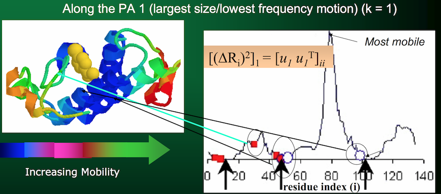
Side, but important, note: the eigenvalues (and corresponding eigenvectors) are sorted in descending order in $\Lambda$. Therefore, the first eigenvalue (and its corresponding eigenvector) will represent the lowest-frequency motion, or the largest fluctuation amplitude.

Aka, the part of the protein that moves the most.

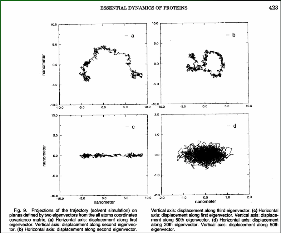
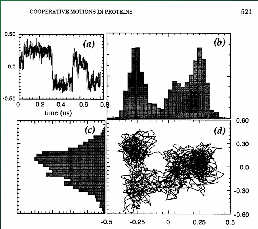
You can use the top handful of principal components to see exactly how the protein moves:

Problem

This all sounds well and good. Problem is, computing eigenvalues and eigenvectors ain't cheap.

We've discussed how $N$ (the number of residues) and $m$ (the number of snapshots) can both get extremely large.

Unless you get into highly sophisticated computing environments, your average SciPy eigen-solver (yep, SciPy has an eigensolver!) runs in $O(n^3)$.

That's fine when $n$ is small, not so fine when $n$ is in the hundreds of thousands or millions.

Singular Value Decomposition (SVD)

Think of SVD as a sort of half-sibling to PCA. In the very specific circumstance where you want to compute a covariance matrix, SVD short-circuits that process and can give you a little performance boost.

Now we don't have to compute the full covariance matrix, just the trajectory matrix $A$:

Similar to PCA, SVD will break down the matrix of interest into three constituent components that have direct biological interpretations. Specifically, we represent our trajectory matrix $A$ as

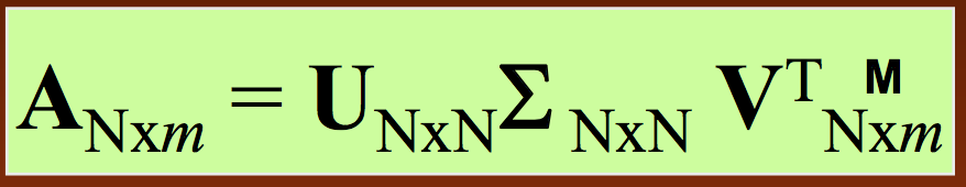
• As before, $U$ is the matrix of principal axis (only now they're called singular vectors instead of eigenvectors)
• Also as before, $\Sigma$ is a diagonal matrix of fluctuation amplitudes (now called singular values instead of eigenvalues)
• The columns of $\Sigma V^T$ are the conformation vectors in the snapshot spanned by the axes $u_i$ for each residue

Let's look at it visually. First, we have our trajectory matrix $A$ of $N$ residues over $m$ time points or snapshots:

From the SVD, one of the parameters we get back is the matrix $V^T$, the rows of which give the displacements along each principal axis (with columns indicating displacement at each time step):

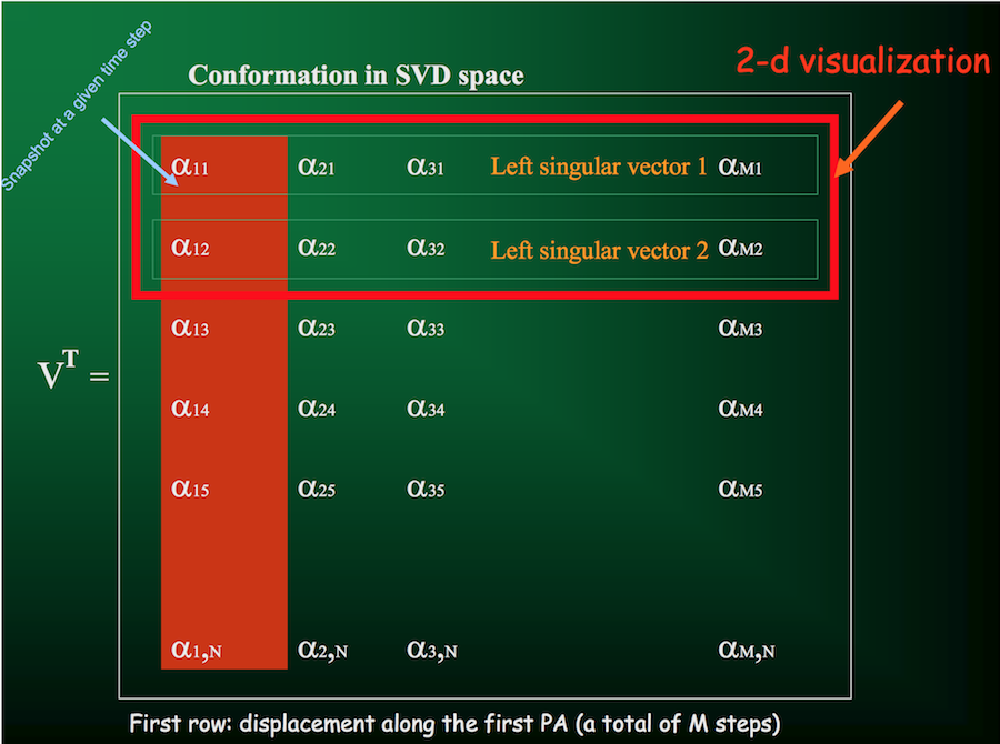
Which you can then use to directly visualize the motion along the principal axes:

Summary of SVD and PCA

These techniques decompose the trajectory into a collection of modes of the protein, sorted in order of significance.

You can use these modes to reconstruct the trajectory based on the dominant modes.

These modes are robust: they are invariant and do not depend on the details of the model or force field.

These modes are also relevant to biological function: you can see what conformations your protein spends most of its time in.

Administrivia

• Assignment 4 is out today! Due in two weeks.

• Final project proposals are due in three weeks!
  • 1 page, maximum
  • Succinctly describe the problem you want to work on, and how you plan to answer it
  • Emphasize the computational approach you want to take
  • Any references

• Have a great spring break!!