Lecture 14: Hidden Markov Models
CBIO (CSCI) 4835/6835: Introduction to Computational Biology
Part 0: A few notes on Assignments 1 and 2
Common mistake 1: loops
What's wrong with this method of looping?
some_list = [3, 5, 1, 7, 1, 2]
for i in some_list:
    i += 1
Be careful not to confuse list elements with list indices.
Common mistake 2: testing code
A lot of instances where tests failed because of syntax errors in the original code.
How to test code in JupyterHub
Overview and Objectives
Today, we'll cover our first true computational modeling algorithm: Hidden Markov Models (HMMs). These are very sophisticated techniques for learning and predicting information that comes to you in some kind of sequence, whether it's an amino acid primary structure, a time-lapse video of molecules being trafficked through cells, or the construction schedule of certain buildings on the UGA campus. By the end of this lecture, you should be able to:
- Define HMMs and why they can be useful in biological sequence alignment
- Describe the assumptions HMMs rely on, and the parameters that have to be learned for an HMM to function
- Recall the core algorithms associated with training an HMM
- Explain the weaknesses of HMMs
Part 1: CG-islands and Casinos
- Given four possible nucleotides (A, T, C, and G), how probable is one of them?
- How probable is a dinucleotide pair, aka any two nucleotides appearing one right after the other?
- As we discussed in last week's lecture, these raw probabilities aren't reflected in the real world
- In particular,
CGis typically underrepresented, clocking in at a frequency considerably less than the "expected" $\frac{1}{16}$
CG-islands
CG is the least frequent dinucleotide (why?).
- The
Cis easily methylated, after which it has a tendency to mutate into aT.
- However, methylation is suppressed around genes in a genome, so
CGwill appear at relatively high frequencies within theseCG-islands.
Finding CG-islands, therefore, is an important biological problem!
The Fair Bet Casino
Let's say you've wandered into a casino, hoping to make enough money to keep you from ever having to write another sequence alignment function using dynamic programming.
This is the Fair Bet Casino: the game is to flip two coins: a fair coin (F) and a biased coin (B).
- Only one of the coins is ever flipped at a time, the outcome of which is always either Heads (H) or Tails (T).
- The fair coin F will give Heads or Tails with equal probability (0.5), so $P(H | F) = P(T | F) = \frac{1}{2}$.
- The biased coin B will give Heads with probability 0.75, so $P(H|B) = \frac{3}{4}$ and $P(T|B) = \frac{1}{4}$.
- The dealer is a sly crank: he'll change between F and B with probability 0.1, so you never actually know which coin he's using.
How can we tell whether the dealer is using F or B?
The "Decoding Problem"
Given: A sequence of coin flips, such as HHHHHHHHHH or HTHTHTHTHT.
We need to be able to "grade" the sequence of coin flips and assign the "most likely" corresponding sequence of Fair or Biased coins making each flip.
We are, in effect, decoding the observed sequence (Heads or Tails) to recover the underlying state (Fair or Biased).
The Simple dog Case
Let's start with an easy case: the dealer never switches coins. Our problem can then be formalized as follows:
- Representing the sequence of coin flips as $x$, $P(x | F)$ is the probability of generating the sequence given the dealer is using the Fair coin
- Similarly, $P(x | B)$ is the probability of generating the sequence $x$ given the dealer is using the Biased coin
We can compute this directly!
Let's say we have
- A sequence of length $n$
- $k$ of the elements are Heads
- $n - k$ are Tails
$P(x | F) = \prod_{i = 1}^n \frac{1}{2} = \left(\frac{1}{2}\right)^k$
So what would the probability using a Biased coin be?
$P(x | B) = \prod_{i = 1}^n \left(\frac{3}{4}\right)^k \left(\frac{1}{2}\right)^{n - k} = \frac{3^k}{4^n}$
So if we made a couple of examples...
Example 1: HTHTHT has a length of 6, with 3 Heads and 3 Tails.
- $P(x | F) = \left(\frac{1}{2}\right)^6$, or 0.15625 (roughly 15.5%)
- $P(x | B) = \frac{3^3}{4^6}$, or 0.006592 (roughly 0.65%)
Which is more likely?
Example 2: HHHHHH has a length of 6, with 6 Heads and 0 Tails.
- $P(x | F) = \left(\frac{1}{2}\right)^6$, or 0.15625 (roughly 15.5%)
- $P(x | B) = \frac{3^6}{4^6}$, or 0.1779785 (roughly 17.8%)
Which is more likely?
Part 2: The Anatomy of HMMs
HMMs can be viewed as "machines" with $k$ hidden states.
Depending on what state the HMM is in, it can "emit" different outputs from an alphabet of all possible outputs--we'll call this alphabet $\Sigma$.
- Each hidden state has its own probabilities for what kind of outputs it likes to emit.
- The HMM can also switch between hidden states with some probability.
While in a certain state, the HMM asks itself two questions:
- What state should I move to next? (it could "move" to the same state it's currently in)
- What symbol from the alphabet $\Sigma$ should I emit?
Hidden States
The hidden states (which give HMMs their name, Hidden Markov Models) are the key component and the part of HMMs that make building them tricky.
We don't know whether the dealer is using a Fair or Biased coin; we don't know whether this portion of an amino acid sequence is an $\alpha$-helix or a $\beta$-sheet; we don't know whether this portion of the genome is a CG island.
The goal of decoding with HMMs is to make the best possible guess as to the sequence of hidden states, given the sequence of emitted symbols.
HMM Parameters
Its parameters are to an HMM what our genomes are to us: they're essentially the genetic makeup that distinguishes one HMM from another.
- $\Sigma$: We've already seen this: it's the set of $m$ possible emission symbols (for an amino acid sequence, this is the amino acid symbols; for a genome, this is the nucleotides; for the Fair Bet Casino, this is the sequence of Heads or Tails).
- $Q$: This is the set of $k$ hidden states (think of it as a list).
- $A$: This is a $k \times k$ matrix containing probabilities of switching between hidden states.
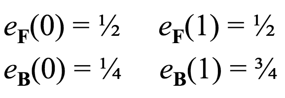
- $E$: This is a $k \times m$ matrix containing probabilities of emitting a certain symbol from $\Sigma$ given that the HMM is in a certain hidden state from $Q$.
A matrix
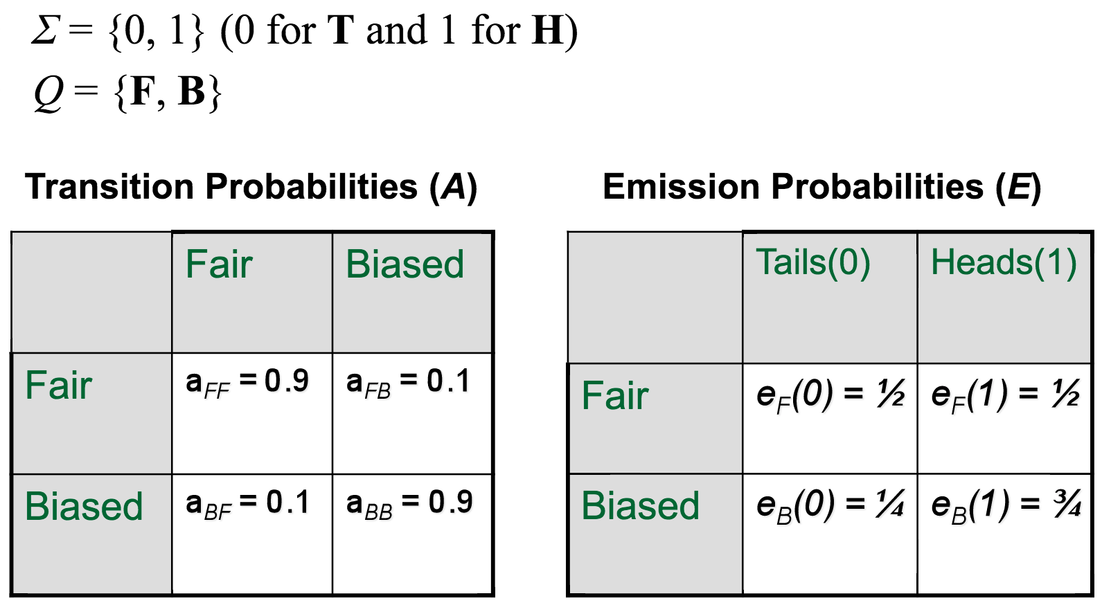
This encodes the probability of switching between hidden states. Using our Fair Bet Casino example, there are only two hidden states, so the matrix will be $2 \times 2$.
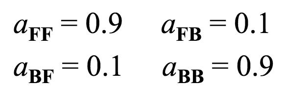
E matrix
This matrix encodes the probabilities of emitting certain symbols, given that the HMM is in a certain hidden state. Using our Fair Bet Casino example, with two hidden states and two possible output symbols, this matrix is also $2 \times 2$.
Taken together, the parameters of our Fair Bet Casino HMM would look something like this:
State Machine
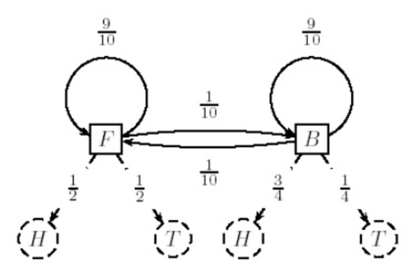
Another perhaps more intuitive perspective would be to view an HMM as a "state machine": each possible state of the HMM is represented as a node in a graph, with arrows connecting the nodes that are weighted based on their probabilities.
Hidden Paths
The observable sequence of emitted symbols (coin flips, amino acids, nucleotides, etc) is one sequence. However, the corresponding sequence of hidden states is known as the hidden paths.
This is usually represented as $\vec{\pi} = \pi_1, ..., \pi_n$.
- (Note: both the hidden path and the observed sequence have the same length, $n$)
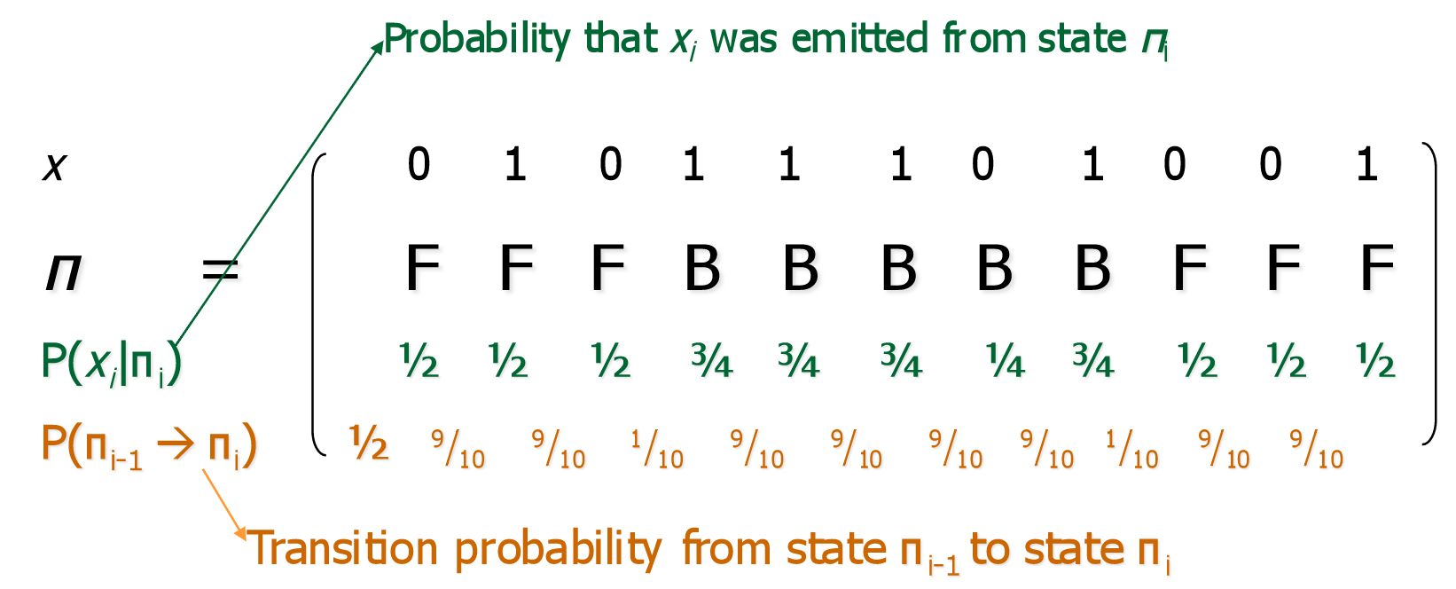
Consider the sequence $x =$ 01011101001 and the hidden path $\vec{\pi} =$ FFFBBBBBFFF. This is how we would list out the probabilities:
Part 3: The Decoding Algorithm
This is the question you'll most often ask of HMMs: given a set of observed sequences, find the optimal hidden path that would have generated the observed sequences.
Formally, this is defined as the following:
- Input: A sequence of observations $\vec{x} = x_1, ..., x_n$ generated by an HMM $M(\Sigma, Q, A, E)$
- Output: A hidden path $\vec{\pi} = \pi_1, ..., \pi_n$ that maximizes $P(x | \pi)$ over all possible hidden paths $\vec{\pi}$
Any ideas?
Who was Andrew Viterbi?
Andrew Viterbi used the the Manhattan edit graph model to solve the decoding problem!
Yep, dynamic programming is back!
Use the same matrix abstraction as before, except instead we only have one sequence of length $n$, and then the other axis is used for the $k$ hidden states.
It looks something like this:
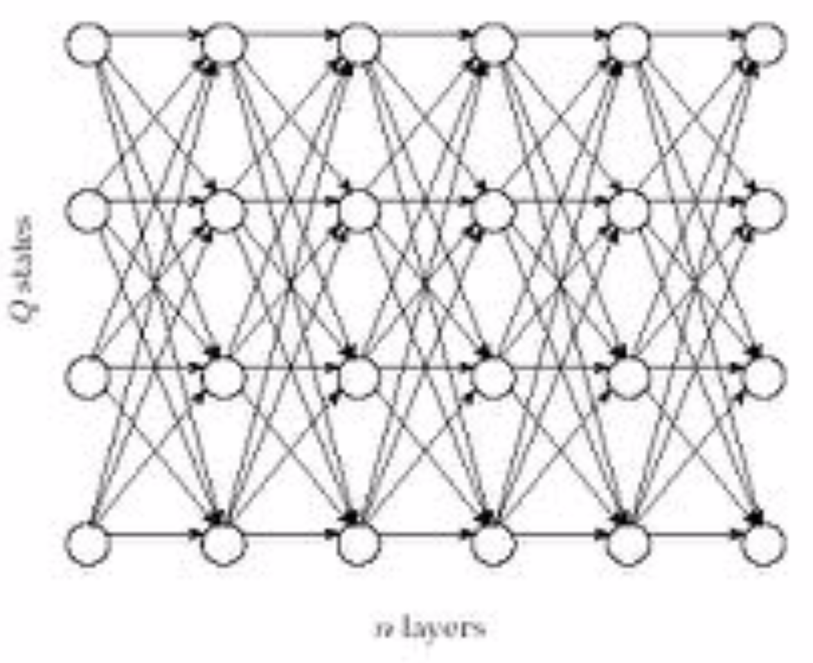
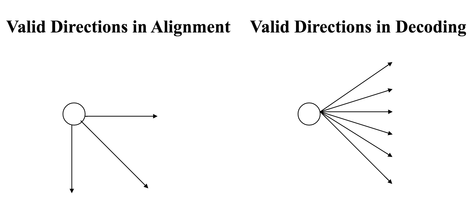
So, instead of having one of 3 decisions at each vertex--insertion, deletion, or match/mutation--we have one of $k$ decisions:
Properties of the Viterbi algorithm
Each possible path through the graph has probability $P(x | \pi)$.
- You're picking a specific hidden path through the graph, so you've fixed $\pi$, and you already know the observed sequence $x$, so that makes the probability straightforward to compute.
The Viterbi algorithm finds the path that gives the maximal possible $P(x | \pi)$, over all possible paths through the graph.
- Consequently, this algorithm has $\mathcal{O}(nk^2)$ runtime complexity (why?)
Part 4: The Forward-Backward Algorithm
This is the question you'll ask of HMMs second in frequency only to the decoding problem: given a set of observed sequences, compute the probability the system was in a certain state at a certain time.
Formally, this is defined as the following:
- Input: A sequence of observations $\vec{x} = x_1, ..., x_n$ generated by an HMM $M(\Sigma, Q, A, E)$
- Output: The probability the HMM was in state $k$ when it emitted symbol $x_i$, or $P(\pi_i = k | x)$.
Any ideas?
Who was Forward-Backward?
Dunno, but this question is answered using a combination of two algorithms: the forward algorithm, and the backward algorithm.

The Forward Algorithm
First, let's define the forward probability as $f_{k, i}$: the probability of emitting a prefix $x_1, ..., x_i$ and reaching state $\pi = k$.
Put another way, this means
- we've already observed (read: we're given) a subsequence of $i$ out of the $n$ symbols: $x_1$ through $x_i$
- we're asking the probability of having reached state $k$ (whatever that is)
[Hopefully] Easy way to remember: we've fixed the first $i$ symbols, but we have to move forward to see the rest.
The Backward Algorithm
Next, we'll define the backward probability as $b_{k, i}$: the probability of being in state $\pi_i = k$, and emitting the suffix $x_{i + 1}, ..., x_n$.
Put another way, we're now looking at
- a system where we now assume (read: we're given) that we've observed the other subsequence of symbols, $x_{i + 1}$ through the end $x_n$
- asking for the probability that starting in state $k$ (whatever that is) would have then generated the aforementioned suffix
[Hopefully] Easy way to remember: we've fixed the last $n - i$ symbols, but have to move backward to get the probability of state $k$.
Backward-Forward Probability
Asking at any given coin flip whether the casino dealer is using a fair or biased coin is, in fact, a function of both the forward and the backward probabilities.
Formally:

(does this look familiar???)
Part 5: Why HMMs?

Profile HMMs
Let's say we're interested in finding a distant cousin of functionally related protein sequences in a family.
This family has diverged so much that pairwise (e.g. Hamming) comparisons are weak, and may therefore fail a statistical significance test.
However, these weak similarities may show up across many members of the family, indicating a correlation.
The goal, then, is to align all members of the family at once.
A family of related proteins can be represented by their multiple alignment and the corresponding profile (hence, the name).
Aligned DNA sequences can be represented as a $4 \times n$ profile matrix, reflecting the frequencies of nucleotides in every aligned position.

Similarly, a protein family can be represented using a $20 \times n$ profile representing amino acid frequencies.
Multiple alignment of a protein family can show variations in conservation along the length of the protein:
- For example, after aligning many globin proteins, biologists recognized that the helices region in globins are far more conserved than others
A profile HMM, then, is a probabilistic representation of a multiple alignment.
This model can then be used to find and score less obvious potential matches of new protein sequences to find distant family members.
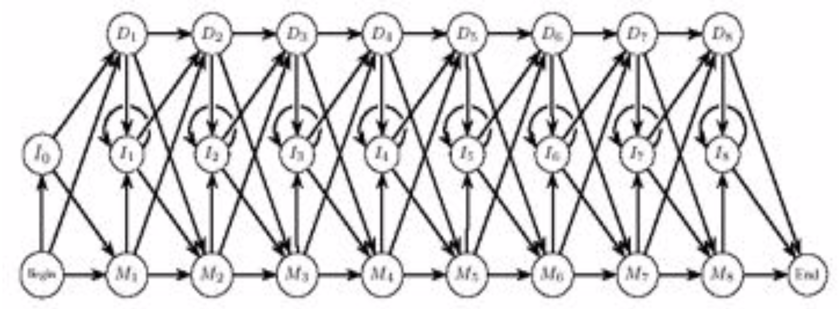
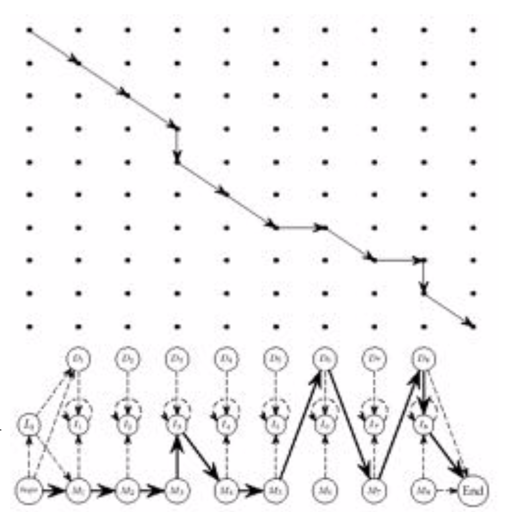
Consists of three states (any guesses?):
- Match states $M_1, ..., M_n$
- Insertion states $I_0, ..., I_n$
- Deletion states $D_1, ..., D_n$
Comparison to dynamic programming
Our walk through the profile HMM is pretty much identical to a walk along the Manhattan edit graph:
How to build a Profile HMM
In four easy steps!
1: Use BLAST to separate a protein database into families of related proteins.
2: Construct a multiple alignment for each protein family.
3: Construct a profile HMM and optimize the parameters of the model (transition and emission probabilities).
4: Align the target sequence (the one you're not sure about) against each profile HMM to find the best fit between the target sequence and a particular HMM
What problem is #4 solving?
Modelilng globin proteins
Globins represent a large collection of protein sequences.
400 globin sequences were randomly selected from all globins and used to construct a multiple alignment.
Multiple alignment was used to train a profile HMM.
Another 625 globin proteins (not used to train the profile HMM) were selected, along with a few hundred other non-globin proteins chosen randomly.
Guess which group--the globins or non-globins--scored better against the profile HMM?
Great way to separate and identify families of proteins; in this case, separate (automatically!) globins and non-globins.
Administrivia
- How is Assignment 3 going? Due Thursday by 11:59pm.
- Speaking of Assignment 3: ignore Question 3, parts E and F. Those are now considered extra credit.
- If you're having trouble with the assignments, please come to office hours! (Tuesdays and Fridays)
- If you're concerned about your performance on the first two assignments, please get in touch with me. Still plenty of time left to ace the course!
Additional Resources
- Matthes, Eric. Python Crash Course, Chapter 10. 2016. ISBN-13: 978-1593276034
- Model, Mitchell. Bioinformatics Programming Using Python, Chapter 2. 2010. ISBN-13: 978-0596154509