Lecture 2: Python Crash Course
CSCI 4360/6360: Data Science II
Part 1: Python Background
Python as a language was implemented from the start by Guido van Rossum. What was originally something of a snarkily-named hobby project to pass the holidays turned into a huge open source phenomenon used by millions.
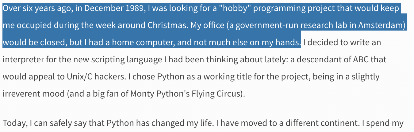
Python's history
The original project began in 1989.
Release of Python 2.0 in 2000
Release of Python 3.0 in 2008
Latest stable release of these branches are 2.7.13--which Guido emphatically insists is the final, final, final release of the 2.x branch--and 3.6.2.
You're welcome to use whatever version you want, just be aware: the AutoLab autograders will be using 3.6.x (unless otherwise noted).
Python, the Language
Python is an intepreted language.
- Contrast with compiled languages
- Performance, ease-of-use
- Modern intertwining and blurring of compiled vs interpreted languages
Python is a very general language.
- Not designed as a specialized language for performing a specific task. Instead, it relies on third-party developers to provide these extras.
Instead, as Jake VanderPlas put it:
"Python syntax is the glue that holds your data science code together. As many scientists and statisticians have found, Python excels in that role because it is powerful, intuitive, quick to write, fun to use, and above all extremely useful in day-to-day data science tasks."
Part 2: Language Basics
The most basic thing possible: Hello, World!
print("Hello, world!")
Yep, that's all that's needed!
(Take note: the biggest different between Python 2 and 3 is the print function: it technically wasn't a function in Python 2 so much as a language construct, and so you didn't need parentheses around the string you wanted printed; in Python 3, it's a full-fledged function, and therefore requires parentheses)
Variables and Types
Python is dynamically-typed, meaning you don't have to declare types when you assign variables. Python is also duck-typed, a colloquialism that means it infers the best-suited variable type at runtime ("if it walks like a duck and quacks like a duck...")
x = 5
type(x)
y = 5.5
type(y)
It's important to note: even though you don't have to specify a type, Python still assigns a type to variables. It would behoove you to know the types so you don't run into tricky type-related bugs!
x = 5 * 5
What's the type for x?
type(x)
y = 5 / 5
What's the type for y?
type(y)
There are functions you can use to explicitly cast a variable from one type to another:
x = 5 / 5
type(x)
y = int(x)
type(y)
z = str(y)
type(z)
Data Structures
There are four main types of built-in Python data structures, each similar but ever-so-slightly different:
- Lists (the Python workhorse)
- Tuples
- Sets
- Dictionaries
(Note: generators and comprehensions are worthy of mention; definitely look into these as well)
Lists are basically your catch-all multi-element data structure; they can hold anything.
some_list = [1, 2, 'something', 6.2, ["another", "list!"], 7371]
print(some_list[3])
type(some_list)
Tuples are like lists, except they're immutable once you've built them (and denoted by parentheses, instead of brackets).
some_tuple = (1, 2, 'something', 6.2, ["another", "list!"], 7371)
print(some_tuple[5])
type(some_tuple)
Sets are probably the most different: they are mutable (can be changed), but are unordered and can only contain unique items (they automatically drop duplicates you try to add). They are denoted by braces.
some_set = {1, 1, 1, 1, 1, 86, "something", 73}
some_set.add(1)
print(some_set)
type(some_set)
Finally, dictionaries. Other terms that may be more familiar include: maps, hashmaps, or associative arrays. They're a combination of sets (for their key mechanism) and lists (for their value mechanism).
some_dict = {"key": "value", "another_key": [1, 3, 4], 3: ["this", "value"]}
print(some_dict["another_key"])
type(some_dict)
Dictionaries explicitly set up a mapping between a key--keys are unique and unordered, exactly like sets--to values, which are an arbitrary list of items. These are very powerful structures for data science-y applications.
Slicing and Indexing
Ordered data structures in Python are 0-indexed (like C, C++, and Java). This means the first elements are at index 0:
print(some_list)
index = 0
print(some_list[index])
However, using colon notation, you can "slice out" entire sections of ordered structures.
start = 0
end = 3
print(some_list[start : end])
Note that the starting index is inclusive, but the ending index is exclusive. Also, if you omit the starting index, Python assumes you mean 0 (start at the beginning); likewise, if you omit the ending index, Python assumes you mean "go to the very end".
print(some_list[:end])
start = 1
print(some_list[start:])
Loops
Python supports two kinds of loops: for and while
for loops in Python are, in practice, closer to for each loops in other languages: they iterate through collections of items, rather than incrementing indices.
for item in some_list:
    print(item)
- the collection to be iterated through is at the end (
some_list) - the current item being iterated over is given a variable after the
forstatement (item) - the loop body says what to do in an iteration (
print(item))
But if you need to iterate by index, check out the enumerate function:
for index, item in enumerate(some_list):
    print("{}: {}".format(index, item))
while loops operate as you've probably come to expect: there is some associated boolean condition, and as long as that condition remains True, the loop will keep happening.
i = 0
while i < 10:
    print(i)
    i += 2
IMPORTANT: Do not forget to perform the update step in the body of the while loop! After using for loops, it's easy to become complacent and think that Python will update things automatically for you. If you forget that critical i += 2 line in the loop body, this loop will go on forever...
Another cool looping utility when you have multiple collections of identical length you want to loop through simultaneously: the zip() function
list1 = [1, 2, 3]
list2 = [4, 5, 6]
list3 = [7, 8, 9]

for x, y, z in zip(list1, list2, list3):
    print("{} {} {}".format(x, y, z))
This "zips" together the lists and picks corresponding elements from each for every loop iteration. Way easier than trying to set up a numerical index to loop through all three simultaneously, but you can even combine this with enumerate to do exactly that:
for index, (x, y, z) in enumerate(zip(list1, list2, list3)):
    print("{}: ({}, {}, {})".format(index, x, y, z))
Conditionals
Conditionals, or if statements, allow you to branch the execution of your code depending on certain circumstances.
In Python, this entails three keywords: if, elif, and else.
grade = 82
if grade > 90:
    print("A")
elif grade > 80:
    print("B")
else:
    print("Something else")
A couple important differences from C/C++/Java parlance:
- NO parentheses around the boolean condition!
- It's not "
else if" or "elseif", just "elif". It's admittedly weird, but it's Python
Conditionals, when used with loops, offer a powerful way of slightly tweaking loop behavior with two keywords: continue and break.
The former is used when you want to skip an iteration of the loop, but nonetheless keep going on to the next iteration.
list_of_data = [4.4, 1.2, 6898.32, "bad data!", 5289.24, 25.1, "other bad data!", 52.4]

for x in list_of_data:
    if type(x) == str:
        continue

    # This stuff gets skipped anytime the "continue" is run
    print(x)
break, on the other hand, literally slams the brakes on a loop, pulling you out one level of indentation immediately.
import random

i = 0
iters = 0
while True:
    iters += 1
    i += random.randint(0, 10)
    if i > 1000:
        break

print(iters)
File I/O
Python has a great file I/O library. There are usually third-party libraries that expedite reading certain often-used formats (JSON, XML, binary formats, etc), but you should still be familiar with input/output handles and how they work:
text_to_write = "I want to save this to a file."
f = open("some_file.txt", "w")
f.write(text_to_write)
f.close()
This code writes the string on the first line to a file named some_file.txt. We can read it back:
f = open("some_file.txt", "r")
from_file = f.read()
f.close()
print(from_file)
Take note what changed: when writing, we used a "w" character in the open argument, but when reading we used "r". Hopefully this is easy to remember.
Also, when reading/writing binary files, you have to include a "b": "rb" or "wb".
Functions
A core tenet in writing functions is that functions should do one thing, and do it well.
Writing good functions makes code much easier to troubleshoot and debug, as the code is already logically separated into components that perform very specific tasks. Thus, if your application is breaking, you usually have a good idea where to start looking.
WARNING: It's very easy to get caught up writing "god functions": one or two massive functions that essentially do everything you need your program to do. But if something breaks, this design is very difficult to debug.
Homework assignments will often require you to break your code into functions so different portions can be autograded.
Functions have a header definition and a body:
def some_function():  # This line is the header
    pass              # Everything after (that's indented) is the body
This function doesn't do anything, but it's perfectly valid. We can call it:
some_function()
Not terribly interesting, but a good outline. To make it interesting, we should add input arguments and return values:
def vector_magnitude(vector):
    d = 0.0
    for x in vector:
        d += x ** 2
    return d ** 0.5
v1 = [1, 1]
d1 = vector_magnitude(v1)
print(d1)
v2 = [53.3, 13.4]
d2 = vector_magnitude(v2)
print(d2)
NumPy Arrays
If you looked at our previous vector_magnitude function and thought "there must be an easier way to do this", then you were correct: that easier way is NumPy arrays.
NumPy arrays are the result of taking Python lists and adding a ton of back-end C++ code to make them really efficient.
Two areas where they excel: vectorized programming and fancy indexing.
Vectorized programming is perfectly demonstrated with our previous vector_magnitude function: since we're performing the same operation on every element of the vector, NumPy allows us to build code that implicitly handles the loop
import numpy as np

def vectorized_magnitude(vector):
    return (vector ** 2).sum() ** 0.5
v1 = np.array([1, 1])
d1 = vectorized_magnitude(v1)
print(d1)
v2 = np.array([53.3, 13.4])
d2 = vectorized_magnitude(v2)
print(d2)
We've also seen indexing and slicing before; here, however, NumPy really shines.
Let's say we have some super high-dimensional data:
X = np.random.random((500, 600, 250))
We can take statistics of any dimension or slice we want:
X[:400, 100:200, 0].mean()
X[X < 0.01].std()
X[:400, 100:200, 0].mean(axis = 1)
Part 3: Document Classification with Python
We'll end our Python crash-course with a bit of a review from 3360 or your previous intro-to-ML experience: document classification with Naive Bayes and Logistic Regression.
Bag of words
Hopefully you're familiar with this abstraction for modeling documents.
This model assumes that each word in a document is drawn independently from a multinomial distribution over possible words (a multinomial distribution is a generalization of a Bernoulli distribution to multiple values). Although this model ignores the ordering of words in a document, it works surprisingly well for a number of tasks, including classification.
In short, it says: word order doesn't matter nearly as much--or perhaps, at all--as word frequency.

Naive Bayes
With any (discriminative) classification problem, you're asking: what's the probability of a label given the data? In our document classification example, this question is: what is the probability of the document class, given the document itself?
Formally, for a document $x$ and label $y$: $P(y | x)$
If we're using individual word counts as features ($x_1$ is word 1, $x_2$ is word 2, and so on), then by the rules of conditional probability, this probability would expand into something like this:
This is, for all practical purposes, intractable. Hence, "naive": we make each word conditionally independent of the others, given the label:
For any given word $x_i$ then, the original problem reduces to:
And since the denominator is the same across all documents, we can effectively ignore it as a constant, thereby giving us a decision:
If you really want to dig into what makes Naive Bayes an improvement over the "optimal Bayes classifier", you can count exactly how many parameters are required in either case.
We'll take the simple example: the decision variable $Y$ is boolean, and the observations $X$ have $n$ attributes, each of which is also boolean. Formally, that looks like this:
$$ \theta_{ij} = P(X = x_i | Y = y_i) $$where $i$ takes on $2^n$ possible values (one for each of the possible combinations of boolean values in the array $X$, and $j$ takes on 2 possible values (true or false). For any fixed $j$ the sum over $i$ of $\theta_{ij}$ has to be 1 (probability). So for any particular $y_j$, you have the $2^{n}$ values of $x_i$, so you need $2^n - 1$ parameters. Given two possible values for $j$ (since $Y$ is boolean!), we must estimate a total of $2 (2^n - 1)$ such $\theta_{ij}$ parameters.
This is a problem!
This means that, if our observations $X$ have three attributes--3-dimensional data--we need 14 distinct data points at least, one for each possible boolean combination of attributes in $X$ and label $Y$. It gets exponentially worse as the number of boolean attributes increases--if $X$ has 30 boolean attributes, we'll have to estimate 30 billion parameters.
This is why the conditional independence assumption of Naive Bayes is so critical: more than anything, it substantially reduces the number of required estimated parameters. If, through conditional independence, we have
$$ P(X_1, X_2, ..., X_n | Y) = \Pi_{i = 1}^n P(X_i | Y) $$or, to illustrate more concretely, observations $X$ with 3 attributes each
$$ P(X_1, X_2, X_3 | Y) = P(X_1 | Y) P(X_2 | Y) P(X_3 | Y) $$we've just gone from requiring the aforementioned 14 parameters, to 6!
Formally: we've gone from requiring $2(2^n - 1)$ parameters to $2n$.
Naive Bayes is a fantastic algorithm and works well in practice. However, it has some important drawbacks to be aware of:
- Data may not be conditionally independent. The easiest example of this: replicating a single observation multiple times. These are clearly dependent entities, but Naive Bayes will treat them as independent of each other, given the class label. In practice this isn't a common occurrence but can happen.
- What about continuous attributes? We've only looked so far at data with boolean attributes; most data, including documents, are not boolean. Rather, they are continuous. We can fairly easily modify Naive Bayes to Gaussian Naive Bayes, where each attribute is an i.i.d. Gaussian, but this introduces new problems: now we're assuming our data are Gaussian, which like conditional independence, may not be true in practice.
- Observing data in testing that was not observed in training. With the document classification example, training the Naive Bayes parameters essentially consists of word counting. However, what happens when you encounter a word $X_i$ in a test set for which you do not have a corresponding $P(X_i | Y)$? By default, this sets a probability of 0, but this is problematic in a Naive Bayes setting: since you're computing $P(X_1 | Y) P(X_2 | Y) ... P(X_n | Y)$ for a document, a single probability of 0 in that string of multiplication nukes the entire statement!
Logistic Regression
Logistic regression is a bit different. Rather than estimating the parametric form of the data $P(x_i | y)$ and $P(y)$ in order to get to the posterior $P(y | x)$, here we're learning the decision boundary $P(y | x)$ directly.
Ideally we want some kind of output function between 0 and 1--so let's just go with the logit
%matplotlib inline
import matplotlib.pyplot as plt

x = np.linspace(-5, 5, 100)
y = 1 / (1 + np.exp(-x))

plt.plot(x, y)

We just adapt the logit function to work our document features $x_i$, and some weights $w_i$:
Then finding $P(Y = 1 | X)$ is just $1 - P(Y = 0 | X)$, or
This second equation, for $P(Y = 1 | X)$, arises directly from the fact that these two terms must sum to 1. Write it out yourself if you need convincing!
So how do we train a logistic regression model? Here's where things get a tiny bit trickier than Naive Bayes.
In Naive Bayes, the bag-of-words model was 90% of the classifier. Sure, we needed some marginal probabilities and priors, but the word counting was easily the bulk of it.
Here, the word counting is still important, but now we have this entire array of weights we didn't have before. These weights correspond to feature relevance--how important the features are to prediction. In Naive Bayes we just kind of assumed that was implicit in the count of the words--higher counts, more relevance. But logistic regression separates these concepts, meaning we now have to learn the weights on our own.
We have our training data: $\{(X^{(j)}, y^{(j)})\}_{j = 1}^n$, and each $X^{(j)} = (x^{(j)}_1, ..., x^{(j)}_d)$ for $d$ features/dimensions/words.
And we want to learn: $\hat{\textbf{w}} = \textrm{argmax}_{\textbf{w}} \Pi_{j = 1}^n P(y^{(j)} | X^{(j)}, \textbf{w})$
Our conditional log likelihood then takes the form: $l(\textbf{w}) = \textrm{ln} \Pi_j P(y^j | \vec{x}^j, \textbf{w})$

How did we get here?
First, note that the likelihood function is typically formally denoted as
$$ W \leftarrow \textrm{arg max}_W \Pi_l P(Y^l | X^l, W) $$for each training example $X^l$ with corresponding ground-truth label $Y^l$ (they are multipled together because we assume each observation is independent of the other). We include the weights $W$ in this expression because the probability is absolutely a function of the weights, and we want to pick the combination of weights $W$ that make the probability expression as large as possible.
Second, because we're both pragmatic enough to use a short-cut whenever we can and evil enough to know it'll confuse other people, we never actually work directly with the likelihood as stated above. Instead, we work with the log-likelihood, by literally taking the log of the function:
$$ W \leftarrow \textrm{arg max}_W \sum_l \textrm{ln} P(Y^l | X^l, W) $$Recall that the log of a product is equivalent to the sum of logs.
Third, the probability statement $P(Y^l | X^l, W)$ has two main terms, since $Y$ can be either 1 or 0; we want to pick the one with the largest probability. So we expand that term into the following:
$$ l(W) = \sum_l Y^l \textrm{ln} P(Y^l = 1|X^l, W) + (1 - Y^l) \textrm{ln} P(Y^l = 0 | X^l, W) $$where $l(W)$ is our log-likehood function.
Hopefully this looks somewhat familiar to you: it's a lot like finding the expected value $E[X]$ of a discrete random variable $X$, where you take each possible value $X = x$ and multiply it by its probability $P(X = x)$, summing them all together. You can see the case $Y = 1$ on the left, and $Y = 0$ on the right, both being multiplied by their corresponding conditional probabilities.
Hopefully you'll also note: since you're using this equation for training, $Y^l$ will take ONLY 1 or 0, therefore zero-ing out one side of the equation or the other for every single training instance. So that's kinda nice?
Fourth, get ready for some math! If we have
$$ l(W) = \sum_l Y^l \textrm{ln} P(Y^l = 1|X^l, W) + (1 - Y^l) \textrm{ln} P(Y^l = 0 | X^l, W) $$Expand the last term:
$$ l(W) = \sum_l Y^l \textrm{ln} P(Y^l = 1|X^l, W) + \textrm{ln} P(Y^l = 0 | X^l, W) - Y^l \textrm{ln} P(Y^l = 0|X^l, W) $$Combine terms with the same $Y^l$ coefficient (first and third terms):
$$ l(W) = \sum_l Y^l \left[ \textrm{ln} P(Y^l = 1|X^l, W) - \textrm{ln} P(Y^l = 0|X^l, W) \right] + \textrm{ln} P(Y^l = 0 | X^l, W) $$Recall properties of logarithms--when subtracting two logs with the same base, you can combine their arguments into a single log dividing the two:
$$ l(W) = \sum_l Y^l \left[ \textrm{ln} \frac{P(Y^l = 1|X^l, W)}{P(Y^l = 0|X^l, W)} \right] + \textrm{ln} P(Y^l = 0 | X^l, W) $$Now things get interesting--remember earlier where we defined exact parametric forms of $P(Y = 1 | X)$ and $P(Y = 0|X)$? Substitute those back in, and you'll get:
$$ l(W) = \sum_l \left[ Y^l (w_0 + \sum_i^d w_i X_i^l) - \textrm{ln}(1 - \textrm{exp}(w_0 + \sum_i^d w_i X_i^l)) \right] $$which is exactly the equation we had before we started going through these proofs.
Good news! $l(\textbf{w})$ is a concave function of $\textbf{w}$, meaning no pesky local optima.
Bad news! No closed-form version of $l(\textbf{w})$ to find explicit values (feel free to try and take its derivative, set it to 0, and solve; it's a transcendental function, so it has no closed-form solution).
Good news! Concave (convex) functions are easy to optimize!
Maximum of a concave function = minimum of a convex function
- Gradient ascent (concave) = gradient descent (convex)
Gradient: $\nabla_{\textbf{w}} l(\textbf{w}) = \left[ \frac{\partial l(\textbf{w})}{\partial w_0}, ..., \frac{\partial l(\textbf{w})}{\partial w_n} \right] $
Update rule: $w_i^{(t + 1)} = w_i^{(t)} + \eta \frac{\partial l(\textbf{w})}{\partial w_i}$
Which ultimately leads us to gradient ascent for logistic regression.
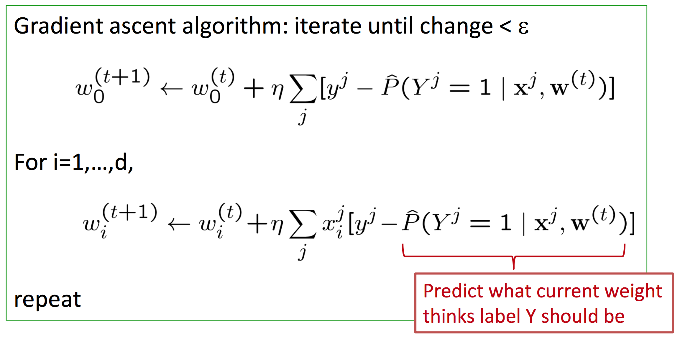
This is Assignment 1!
In addition to going over some basic concepts in probability, Naive Bayes, and Logistic Regression, you'll also implement some document classification code from scratch (don't let me catch anyone using scikit-learn, mmk).
The hardest part in the coding will be implementing gradient descent! It's not a lot of code--especially if you use NumPy vectorized programming--but it will take some sitting-and-thinking-and-whiteboarding time (unless you know this stuff cold already, I suppose)!
There is also some theory and small proofs.
Don't be intimidated. I purposely made this homework tricky both to get an idea of your level of understanding of the topics so I can gauge how to proceed in the course, and also so you have an idea where your weaknesses are.
ASK ME FOR HELP! Helping students is literally my day job. Don't be shy; if you're stuck, reach out for help, both from me AND your student colleagues!
Administrivia
- Assignment 1 is out on AutoLab. This is a warm-up to familiarize you with Python, AutoLab, and to make sure you're up to speed on the basics of machine learning and probability. You'll be implementing Multinomial Naive Bayes and Logistic Regression from first principles. Should be fun! Assignment 1 is due Thursday, August 31 by 11:59pm.
- The first Workshop is Wednesday, August 30. If you have not yet signed up for workshops, please do so here: https://docs.google.com/spreadsheets/d/1SmEhL30kBvjPa6WioR34zM8HP5HuY38N3vGzQEwGVS0/edit#gid=0 (Just FYI: after this weekend, I will auto-assign anyone who has not yet signed up).
- I will be out of town all next week and part of the week after. I agree it's bad timing, but I will be in touch by Slack and email. In the meantime, we'll have guest lecturers discussing their work in different areas of data science, so please be sure to attend if you're at all interested in seeing what different forms data science can take!