Your Presenter:
Christian McDaniel
¶Data Scientist & Software Engineer,
NCR Innovation Lab
¶- Got my Master's in Artificial Intelligence in August 2019
- Conducted my thesis research under Dr. Shannon Quinn on deep learning-based multi-modal neuroimaging research for Parkinson's Disease
- Currently work on Computer Vision-based applications to Retail, Finance, and Hospitality at NCR
Graph Convolutional Networks
Background
- Graph Convolutional Networks are both simple and complex
- They borrow from multiple domains to arrive at an elegant analysis algorithm
- Deep Learning - Convolutional Neural Networks
- Spectral Graph Clustering - Graph Laplacian
- Signal Processing - Fourier Transform

Graph Convolutional Networks
Background
- I.e., the points of the dataset make up the nodes of a graph
- We could just plug in these point to a traditional classification algorithm
- OR we could use the connections between the nodes to cluster the datapoints
- But neither are sufficient, so we'd like to utilize both the features of each node AND the connections between them
| Word Embedding | Molecular Structure | Traffic Routes | Neuronal Networks |
|---|---|---|---|
 |
 |
Graph Convolutional Networks
Background - Convolutional Neural Networks
| _ | _ |
|---|---|
+ Great success with computer vision-based applications |
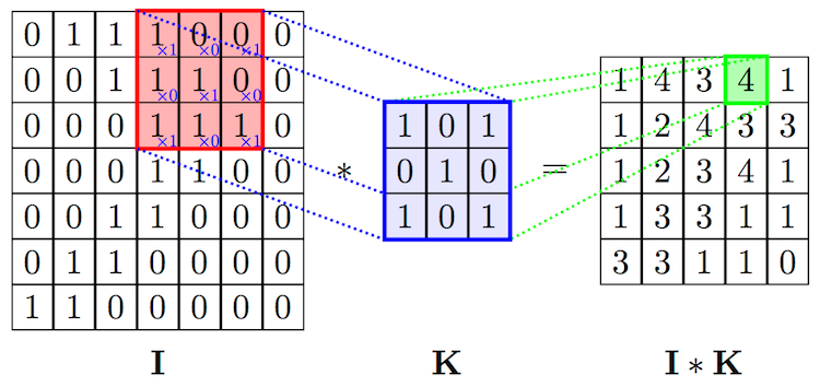 |
Images as Well-Behaved Graphs

Images as Well-Behaved Graphs
| _ | _ |
|---|---|
|
 |
Images as Well-Behaved Graphs
| _ | _ | _ |
|---|---|---|
|
|
 |
Graph Convolutional Networks
- Generalizing the convolution operation for arbitrary graph structures is much more tricky
- We will use some very convenient (and awesome) rules from Signal Processing and Spectral Graph Theory
- Next we'll discuss recent advances improving performance and computational efficiency
- (Semi-Supervised Classification with Graph Convolutional Networks, Kipf & Welling 2016)
Graph Convolutional Networks
Before we learn the ituitions, let's first look at what a simple GCN may look like:
The graph-based convolution:
$Z = \tilde{D}^{\frac{-1}{2}}\tilde{A}\tilde{D}^{\frac{-1}{2}}X\Theta$
Add in a Nonlinear Activation
- Graph structure is encoded directly into the neural network model by incorporating the adjacency matrix: $f(X,A)$
- We can do so by wrapping the above equation in a nonlinear activation function:
$H^{(l+1)} = \sigma(\tilde{D}^{\frac{-1}{2}}\tilde{A}\tilde{D}^{\frac{-1}{2}}H^{l}W^{l})$
- Where $W^{l}$ is a layer-specific trainable weight matrix, $\sigma(\cdot)$ is an activation function, $H^{l} \in \mathbb{R}^{N x F^{l}}$ is the matrix of activations from the $l^{th}$ layer, and $H^{0}=X$
- A two-layer Graph Convolutional Network may look something like
$Z = f(X,A) = \textrm{softmax}(\hat{A} \textrm{ReLU}(\hat{A}XW^{0})W^{1})$
- Where $\hat{A}$ is the precalculated $D^{\frac{-1}{2}}AD^{\frac{-1}{2}}$
So... Where did this implimentation come from??
1. Generalizing the Convolution
- A convolution operation combines one function $f$ with another function $g$ such that the first function is transformed by the other
- In Convolutional Neural Networks, the second function $g$ is learned for a given data set so that the transformations on $f$ are meaningful w.r.t. some class values
- e.g., a set of pixels showing a dog, $f_{d}$ may be transformed to values near $0$
- while a set of pixels showing a cat, $f_{c}$ may be transformed to values near $1$
- Let's see how we might do this for our graph-based data...
Graph Convolutional Networks
Signal Processing
- With the nodes of the graph representing individual examples from the dataset,
- And some data at each node
- E.g.,
- scalar intensity values at each pixel of an image
- feature vectors for higher dimensional data
- We can consider the data values as signals on each node

Graph Convolutional Networks
Signal Processing
- With the nodes of the graph representing individual examples from the dataset,
- And some data at each node
- scalar intensity values at each pixel of an image
- feature vectors for higher dimensional data
- We can consider the data values as signals on each node
- Intuitively, by commuting over the nodes of the graph, we could learn a function $g$ that transforms the values at each node in a meaningful way
- How might we define the "filter" $g$...?
Graph Convolutional Networks
Signal Processing
- With the nodes of the graph representing individual examples from the dataset,
- And some data at each node
- scalar intensity values at each pixel of an image
- feature vectors for higher dimensional data
- We can consider the data values as signals on each node
- The changing of the signals across the edges of the graph resemble the fluctuation of a signal over time
- Borrowing from signal processing, these oscillations could be characterized by their component frequencies, via the Fourier transform
- It just so happens that graphs have their own version of the FT...

Graph Convolutional Networks
The Normalized Graph Laplacian in the Spectral Domain
- The Normalized Graph Laplacian $L$ is a real symmetric positive semidefinite matrix
- $z^{T}Lz \geq 0$ for all columns z
- it has a complete set of orthonormal eigenvectors $\{u_{l}\}_{l=0}^{n−1} \in \mathbb{R}^{n}$ a.k.a. the graph Fourier modes
- and it has the associated ordered real nonnegative eigenvalues $\{λ_{l}\}_{l=0}^{n−1}$, the frequencies of the graph
- $L$ is diagonalized in the Fourier basis $U = [u_{0}, u_{1}, ..., u{n-1}] \in \mathbb{R}^{nxn}$ such that
$L = U^{T} \Lambda U$
- Where $\Lambda = \textrm{diag}([\lambda_{0}, \lambda_{1}, ..., \lambda_{n-1}] \in \mathbb{R}^{nxn})$
I.e.,
$L = I - D^{-1/2} A D^{-1/2} = U^{T} \Lambda U$
Graph Convolutional Networks
The Normalized Graph Laplacian in the Spectral Domain
$L = I - D^{-1/2} A D^{-1/2} = U^{T} \Lambda U$
The Graph Fourier Transform
- The Fourier transform in the graph domain, where eigenvectors denote Fourier modes and eigenvalues denote frequencies of the graph is defined
$\hat{x} = U^{T}x \in \mathbb{R}^{n}$
- As on Euclidean spaces, this transform enables the formulation of fundamental operations.
- E.g., the convolution operation becomes multiplication, and we can define a convolution of a data vector $x$ with a filter $g_{\Theta}$ as
$g_{\Theta} \ast x = U ((U^{T}g_{\Theta}) \bigodot (U^{T}x)) = g_{\Theta}(U \Lambda U^{T})x$
Graph Convolutional Networks
The Normalized Graph Laplacian in the Spectral Domain
$L = I - D^{-1/2} A D^{-1/2} = U^{T} \Lambda U$
The Graph Fourier Transform
$g_{\Theta} \ast x = U ((U^{T}g_{\Theta}) \bigodot (U^{T}x)) = g_{\Theta}(U \Lambda U^{T})x$
- By combining the filters $g_{\Theta}$ with the eigenvalue matrix $\Lambda$, we redefine the task of learning the filter $g$ as learning the Fourier coefficients that define the Fourier function of our graph
$g_{\Theta} \ast x = g_{\Theta}(U \Lambda U^{T})x = U\hat{G}U^{T}x$
- Where $\hat{G} = g_{\Theta}(\Lambda)$ is a diagonal matrix of spectral filter coefficients
Graph Convolutional Networks
The Normalized Graph Laplacian in the Spectral Domain
$L = I - D^{-1/2} A D^{-1/2} = U^{T} \Lambda U$
The Graph Fourier Transform
$g_{\Theta} \ast x = U ((U^{T}g_{\Theta}) \bigodot (U^{T}x)) = g_{\Theta}(U \Lambda U^{T})x$
Signal Processing
$g_{\Theta} \ast x = g_{\Theta}(U \Lambda U^{T})x = U\hat{G}U^{T}x$
- As computing the eigenspectrum of a matrix can be computationally exepensive, we can approximate the Fourier coefficients using a Kth order Chebychev Polynomial
$g_{\Theta}\prime \approx \sum^{K}_{k=0}\Theta\prime_{k}T_{k}(\tilde{\Lambda})$
- Where rescaled $\tilde{\Lambda} = \frac{2}{\lambda_{max}}\Lambda - I$
Graph Convolutional Networks
The Normalized Graph Laplacian in the Spectral Domain
$L = I - D^{-1/2} A D^{-1/2} = U^{T} \Lambda U$
The Graph Fourier Transform
$g_{\Theta} \ast x = U ((U^{T}g_{\Theta}) \bigodot (U^{T}x)) = g_{\Theta}(U \Lambda U^{T})x$
Signal Processing
$g_{\Theta} \ast x = g_{\Theta}(U \Lambda U^{T})x = U\hat{G}U^{T}x$
$g_{\Theta}^{\prime} \approx \sum^{K}_{k=0}\Theta^{\prime}_{k}T_{k}(\tilde{\Lambda})$
- This lets us define
$g_{\Theta} \ast x \approx \sum^{K}_{k=0}\Theta^{\prime}_{k}T_{k}(\tilde{L})x$
- with $\tilde{L} = \frac{2}{\lambda_{max}}L - I$
- The convolution is now $K$-localized, operating only on the nodes a distance of $K$ away from any given node
Graph Convolutional Networks
The Normalized Graph Laplacian in the Spectral Domain
$L = I - D^{-1/2} A D^{-1/2} = U^{T} \Lambda U$
The Graph Fourier Transform and Signal Processing
$g_{\Theta} \ast x = U ((U^{T}g_{\Theta}) \bigodot (U^{T}x)) = g_{\Theta}(U \Lambda U^{T})x = U\hat{G}U^{T}x$
$g_{\Theta} \ast x \approx \sum^{K}_{k=0}\Theta^{\prime}_{k}T_{k}(\tilde{L})x$
Subsequent Computational Advancements
1) In moving toward multi-layer networks, we can remove the explicit Chebychev parameterization by limiting the layer-wise convolution operation to $K=1$
- This makes the function linear w.r.t. $L$
- Prevents overfitting on local neighborhood structures
- Allows deeper models with the same computation, improving modeling capacity
Graph Convolutional Networks
The Normalized Graph Laplacian in the Spectral Domain
$L = I - D^{-1/2} A D^{-1/2} = U^{T} \Lambda U$
The Graph Fourier Transform and Signal Processing
$g_{\Theta} \ast x = U ((U^{T}g_{\Theta}) \bigodot (U^{T}x)) = g_{\Theta}(U \Lambda U^{T})x = U\hat{G}U^{T}x$
$g_{\Theta} \ast x \approx \sum^{K}_{k=0}\Theta^{\prime}_{k}T_{k}(\tilde{L})x$
Subsequent Computational Advancements
1) $K=1$
2) When calculating the rescaled $\tilde{\Lambda}$ and $\tilde{L}$, we can approximate $\lambda_{max} \approx 2$, expecting the neural network paramaters to adapt accordingly during training.
$\tilde{L} = \frac{2}{\lambda_{max}}L - I$, where $L = I - D^{-1/2} A D^{-1/2} \rightarrow \tilde{L} \approx L - I = D^{\frac{-1}{2}}AD^{\frac{-1}{2}}$
$g_{\Theta} \ast x \approx \theta^{\prime}_{0}x + \theta^{\prime}_{1}(L - I)x = \theta^{\prime}_{0}x + \theta^{\prime}_{1}D^{\frac{-1}{2}}AD^{\frac{-1}{2}}x$
- with two free parameters $\lambda^{\prime}_{0}$ and $\lambda^{\prime}_{1}$
Graph Convolutional Networks
The Normalized Graph Laplacian in the Spectral Domain
$L = I - D^{-1/2} A D^{-1/2} = U^{T} \Lambda U$
The Graph Fourier Transform and Signal Processing
$g_{\Theta} \ast x = U ((U^{T}g_{\Theta}) \bigodot (U^{T}x)) = g_{\Theta}(U \Lambda U^{T})x = U\hat{G}U^{T}x$
$g_{\Theta} \ast x \approx \sum^{K}_{k=0}\Theta^{\prime}_{k}T_{k}(\tilde{L})x$
Subsequent Computational Advancements
1) $K=1$
2) $g_{\Theta} \ast x \approx \theta^{\prime}_{0}x + \theta^{\prime}_{1}D^{\frac{-1}{2}}AD^{\frac{-1}{2}}x$
3) We can further constrain the problem to learning a single parameter (per dimension in $x$): $\theta = \theta^{\prime}_{0} = -\theta^{\prime}_{1}$
- This further prevents overfittings and reduces computations
Subsequent Computational Advancements
4) The previous revisions have left $L$ with eigenvalues in $[0,2]$, potentially leading to numerical instabilities and exploding/vanishing gradients due to repeated operations
- A "renormalization trick" has been devised:
$D^{\frac{-1}{2}}AD^{\frac{-1}{2}} \rightarrow \tilde{D}^{\frac{-1}{2}}\tilde{A}\tilde{D}^{\frac{-1}{2}}$
- With $\tilde{A} = A + I$ and $\tilde{D}_{ii} = \sum_{j} \tilde{A}_{ij}$ (i.e., self-loops have been added)
- We generalize this to a signal $X \in \mathbb{R}^{N x P}$ with $P$-dimensional vectors at each node and $F$ filters as
$Z = \tilde{D}^{\frac{-1}{2}}\tilde{A}\tilde{D}^{\frac{-1}{2}}X\Theta$
- Where $\Theta \in \mathbb{R}^{P x F}$ is a matrix of filter coefficients to learn, and $Z \in \mathbb{R}^{N x F}$ is the convolved signal matrix
- This has complexity $\mathcal{O}(|\mathcal{E}|FP)$ where $\mathcal{E}$ is the number of edges in the graph

Graph Convolutional Networks
The graph-based convolution:
$Z = \tilde{D}^{\frac{-1}{2}}\tilde{A}\tilde{D}^{\frac{-1}{2}}X\Theta$
Nonlinear Activation
- Graph structure is encoded directly into the neural network model by incorporating the adjacency matrix: $f(X,A)$
- We can do so by wrapping the above equation in a nonlinear activation function:
$H^{(l+1)} = \sigma(\tilde{D}^{\frac{-1}{2}}\tilde{A}\tilde{D}^{\frac{-1}{2}}H^{l}W^{l})$
- Where $W^{l}$ is a layer-specific trainable weight matrix, $\sigma(\cdot)$ is an activation function, $H^{l} \in \mathbb{R}^{N x F^{l}}$ is the matrix of activations from the $l^{th}$ layer, and $H^{0}=X$
- A two-layer Graph Convolutional Network may look something like
$Z = f(X,A) = \textrm{softmax}(\hat{A} \textrm{ReLU}(\hat{A}XW^{0})W^{1})$
- Where $\hat{A}$ is the precalculated $D^{\frac{-1}{2}}AD^{\frac{-1}{2}}$
""" Github: tkipf/pygcn """
import math
import torch
from torch.nn.parameter import Parameter
from torch.nn.modules.module import Module

class GraphConvolution(Module):
    """
    Simple GCN layer, similar to https://arxiv.org/abs/1609.02907
    """
    def __init__(self, in_features, out_features, bias=True):
        super(GraphConvolution, self).__init__()
        self.in_features = in_features
        self.out_features = out_features
        self.weight = Parameter(torch.FloatTensor(in_features, out_features))
        if bias:
            self.bias = Parameter(torch.FloatTensor(out_features))
        else:
            self.register_parameter('bias', None)
        self.reset_parameters()

    def reset_parameters(self):
        stdv = 1. / math.sqrt(self.weight.size(1))
        self.weight.data.uniform_(-stdv, stdv)
        if self.bias is not None:
            self.bias.data.uniform_(-stdv, stdv)

    def forward(self, input, adj):
        support = torch.mm(input, self.weight)
        output = torch.spmm(adj, support)
        if self.bias is not None:
            return output + self.bias
        else:
            return output
""" Github: tkipf/pygcn """
import torch.nn as nn
import torch.nn.functional as F
from layers import GraphConvolution


class GCN(nn.Module):
    def __init__(self, nfeat, nhid, nclass, dropout):
        super(GCN, self).__init__()

        self.gc1 = GraphConvolution(nfeat, nhid)
        self.gc2 = GraphConvolution(nhid, nclass)
        self.dropout = dropout

    def forward(self, x, adj):
        x = F.relu(self.gc1(x, adj))
        x = F.dropout(x, self.dropout, training=self.training)
        x = self.gc2(x, adj)
        return F.log_softmax(x, dim=1)
Graph Convolutional Networks
Example
- The Cora Dataset
- 2708 Machine Learning papers --> the Nodes
- 7 classes:
- Case_Based
- Genetic_Algorithms
- Neural_Networks
- Probabilistic_Methods
- Reinforcement_Learning
- Rule_Learning
- Theory
- Each paper is cited by at least one other paper --> the Edges
- Each paper is described by the frequency of 1433 unique and meaningful words --> the Features
import pandas as pd

edges    = pd.read_csv('/Users/cm185255/Documents/pygcn/data/cora/cora.cites',sep='\t',header=None,names=["cited paper ID","ID of paper cited"])
features = pd.read_csv('/Users/cm185255/Documents/pygcn/data/cora/cora.content',sep='\t',header=None)

print('Table for the Edges (citations between papers)')
print(edges.head())
print('\nTable for the Features (word counts for each paper; last column = class)')
print(features.head())

...

Table for the Edges (citations between papers)
   cited paper ID  ID of paper cited
0              35               1033
1              35             103482
2              35             103515
3              35            1050679
4              35            1103960

Table for the Features (word counts for each paper; last column = class)
      0     1     2     3     ...  1431  1432  1433                    1434
0    31336     0     0     0  ...     0     0     0         Neural_Networks
1  1061127     0     0     0  ...     0     0     0           Rule_Learning
2  1106406     0     0     0  ...     0     0     0  Reinforcement_Learning
3    13195     0     0     0  ...     0     0     0  Reinforcement_Learning
4    37879     0     0     0  ...     0     0     0   Probabilistic_Methods

[5 rows x 1435 columns]

- ManiReg = Manifold regularization (Belkin et al 2006)
- SemiEmb = semi-supervised embedding (Watson et al, 2012)
- LP = label propagation (Zhu et al, 2003)
- DeepWalk = skip-gram graph embeddings (Perozzi et al, 2014)
- ICA = iterative classification algorithm (Lu & Getoor, 2003)
- Planetois (Yang et al, 2016)
Graph Convolutional Networks
Example #2 - Adding Attention coefficients for whole-graph classification
- Graph Attention Networks (2018)
- Petar Veličković, Guillem Cucurull, Arantxa Casanova, Adriana Romero, Pietro Liò, Yoshua Bengio
- Utilizes self-attention to compute a concise representation of a signal sequence
Graph Convolutional Networks
Example #2 - Adding Attention coefficients for whole-graph classification
At each layer, the features at each node are transformed
$\pmb{h} = \{h_{1}, h_{2}, ..., h_{N}\}, h_{i} \in \mathbb{R}^{F} \rightarrow \pmb{h}^{\prime} = \{h_{1}^{\prime}, h_{2}^{\prime}, ..., h_{N}^{\prime}\}, h_{i}^{\prime} \in \mathbb{R}^{F^{\prime}}$
A shared weight matrix is learned for all nodes, and attention coefficients are calculated to denote importance of every node i to its neighbors j
$e_{ij} = a(\pmb{W}h_{i},\pmb{W}h_{j})$
Where $a(\cdot)$ is an attention mechanism. In our case - a single GCN layer
$\pmb{W} \in \mathbb{R}^{F^{\prime}xF}$
Only the k-nearest neighbors are attended over for each node $i$
- Coefficients are noramalized via softmax
| Anatomical MRI | Diffusion MRI |
|---|---|
  |
  |
Hypothesis:
- Parkinson's disease results in structural and functional brain changes related to decreased dopamine production
- Neuroimaging has shown promise (though limited) for PD detection and research
- Combining insights from multiple modalities may help reveal new discoveries and improve detection
The data
- Anatomical MRI helps identify regions of the brain; doesn't say much about PD pathology
- There are multiple tractography algorithms; each offers unique information about structural connectivity
- Each tractography algorithm generates a new set of features for the same graph
The GCN Implimentation
- The algorithm will need to consolidate data from multiple tractography algorithms
- The outputs from the GCN on each node will need to be consolidated to a single output (PD vs HC) for each graph
Graph Convolutional Networks


Fin!
Questions?